The NLPFDD subroutine approximates derivatives by using the finite-differences method.

See the section Nonlinear Optimization and Related Subroutines for a listing of all NLP subroutines. See Chapter 14 for a description of the arguments of NLP subroutines.

The NLPFDD subroutine can be used for the following tasks:

• If the module "fun" returns a scalar, the NLPFDD subroutine computes the function value f, the gradient vector g, and the Hessian matrix h, all evaluated at the point x0.

• If the module "fun" returns a column vector of function values, the subroutine assumes that a least squares function is specified, and it computes the function vector , the Jacobian matrix , and the crossproduct of the Jacobian matrix at the point x0. Note that in this case, you must set the first element of the par argument to .

If any of the results cannot be computed, the subroutine returns a missing value for that result.

You can specify the following input arguments with the NLPFDD subroutine:

• The "fun" argument refers to a module that returns either a scalar value or a column vector of length . This module returns the value of the objective function or, for least squares problems, the values of the functions that the objective function comprises.

• The x0 argument is a vector of length that defines the point at which the functions and derivatives should be computed.

• The par argument is a vector that defines options and control parameters. Note that the par argument in the NLPFDD call is different from the one used in the optimization subroutines.

• The "grd" argument is optional and refers to a module that returns a vector that defines the gradient of the function at x0. If the fun argument returns a vector of values instead of a scalar, the "grd" argument is ignored.

If the "fun" module returns a scalar, the subroutine returns the following values:

• f is the value of the function at the point x0.

• g is a vector that contains the value of the gradient at the point x0. If you specify the "grd" argument, the gradient is computed from that module. Otherwise, the approximate gradient is computed by a finite difference approximation by using calls of the function module in a neighborhood of x0.

• h is a matrix that contains a finite difference approximation of the value of the Hessian at the point x0. If you specify the "grd" argument, the Hessian is computed by calls of that module in a neighborhood of x0. Otherwise, it is computed by calls of the function module in a neighborhood of x0.

If the "fun" module returns a vector, the subroutine returns the following values:

• f is a vector that contains the values of the functions comprising the objective function at the point x0.

• g is the Jacobian matrix , which contains the first-order derivatives of the functions with respect to the parameters, evaluated at x0. It is computed by finite difference approximations in a neighborhood of x0.

• h is the crossproduct of the Jacobian matrix, . It is computed by finite difference approximations in a neighborhood of x0.

The par argument is a vector of length 3.

• par[1] corresponds to the opt[1] argument in the optimization subroutines. This argument is relevant only to least squares optimization methods, in which case it specifies the number of functions returned by the module "fun". If par[1] is missing or is smaller than 1, it is set to 1.

• par[2] corresponds to the opt[8] argument in the optimization subroutines. It determines what type of approximation is to be used and how the finite difference interval, , is to be computed. See the section Finite-Difference Approximations of Derivatives for details.

• par[3] corresponds to the par[8] argument in the optimization subroutines. It specifies the number of accurate digits in evaluating the objective function. The default is , where is the machine precision.

If you specify a missing value in the par argument, the default value is used.

The NLPFDD subroutine is particularly useful for checking your analytical derivative specifications of the "grd", "hes", and "jac" modules. You can compare the results of the modules with the finite difference approximations of the derivatives of f at the point x0 to verify your specifications.

In the unconstrained Rosenbrock problem (see the section Unconstrained Rosenbrock Function), the objective function is

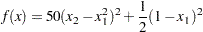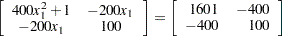
Then the gradient and the Hessian, evaluated at the point , are

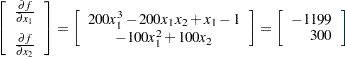The following statements define the Rosenbrock function and use the NLPFDD call to compute the gradient and the Hessian:

start F_ROSEN(x);
   y1 = 10 * (x[2] - x[1] * x[1]);
   y2 =  1 - x[1];
   f  = 0.5 * (y1 * y1 + y2 * y2);
   return(f);
finish F_ROSEN;
x = {2 7};
call nlpfdd(crit, grad, hess, "F_ROSEN", x);
print grad;
print hess;

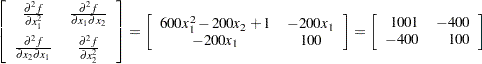
If the Rosenbrock problem is considered from a least squares perspective, the two functions are

Then the Jacobian and the crossproduct of the Jacobian, evaluated at the point , are

The following statements define the Rosenbrock problem in a least squares framework and use the NLPFDD call to compute the Jacobian and the crossproduct matrix. Since the value of the PARMS variable, which is used for the par argument, is 2, the NLPFDD subroutine allocates memory for a least squares problem with two functions, and .

start F_ROSEN(x);
   y = j(2, 1, 0);
   y[1] = 10 * (x[2] - x[1] * x[1]);
   y[2] =  1 - x[1];
   return(y);
finish F_ROSEN;
x     = {2 7};
parms = 2;
call nlpfdd(fun, jac, crpj, "F_ROSEN", x, parms);
print jac;
print crpj;