Variable Transformations
Many statistical analyses assume that the data are normally distributed. If a variable is not normally distributed, it is often possible to improve normality by using an appropriate transformation of the variable. The three transformations used most often for this purpose are the logarithmic, square root, and inverse transformations.
The following steps apply a logarithmic transformation to the driltime variable of the Miningx data set. Because the driltime variable is nonnegative, a logarithmic transformation is well-defined.
-
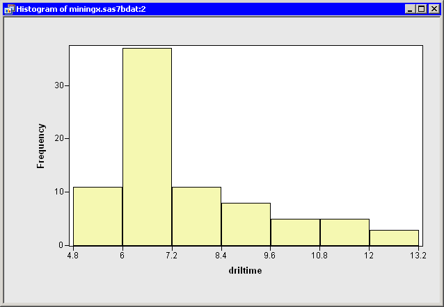
Create a histogram of the
driltimevariable.The histogram is shown in Figure 32.1.
Clearly, the
driltimevariable is not normally distributed. You might explore whether some transformation ofdriltimeis approximately normal. To begin, you might try a logarithmic transformation. -
Select → from the main menu.
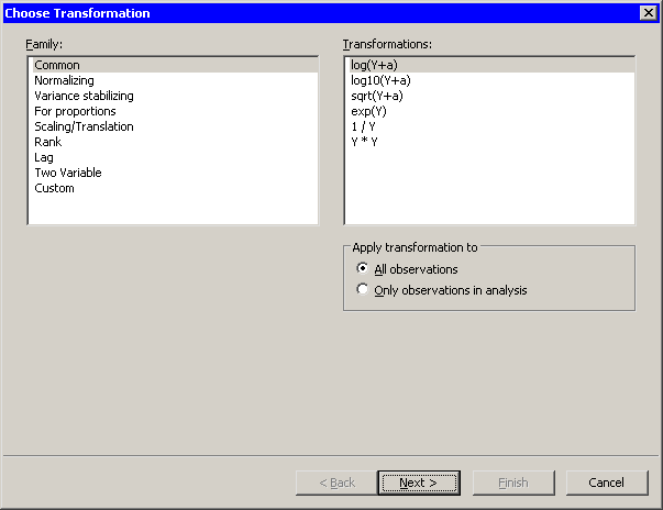
The Variable Transformation Wizard in Figure 32.2 appears.
The first page of the wizard enables you to select a transformation family and a specific transformation within that family. The logarithmic transformation is available from several items in the list, including the family. This transformation is of the form
 , so you need to specify the variable y and the parameter a.
The transformation is highlighted by default. Since this is the desired transformation, you can proceed to the next page of the wizard.
-
Click .
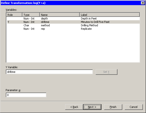
The wizard displays the page shown in Figure 32.3. Note that the transformation appears on the page’s title bar.
-
Select the
driltimevariable, and click .The parameter a is an offset that is useful if your variable contains nonpositive values. For these data, you can accept the default value of 0.
-
Click .
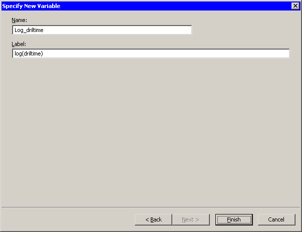
The wizard displays the page shown in Figure 32.4. You can use this page to specify a variable name (and, optionally, a label) for the new variable.
For this example, you can accept the default variable name.
-
Click .
SAS/IML Studio adds the new variable,
Log_driltime, as the last variable in the data set. You can horizontally scroll through the data table to see the variable.To complete this example, you can visualize the distribution of the new variable.
-
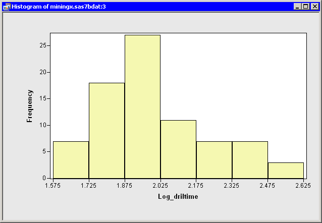
Create a histogram of the
Log_driltimevariable.The histogram shows improved normality, but the transformed data distribution is still skewed to the right. (See Figure 32.5.)