Data Smoothing: Thin-Plate Spline
In this example, you fit a thin-plate spline curve to data in the miningx data set. These data are discussed in Chapter 18: Data Smoothing: Loess. The miningx data set contains 80 observations that correspond to a single test hole in the mining data set. The driltime variable is the time that is required to drill the last five feet of the current depth, in minutes; the hole depth is recorded
in the depth variable.
To fit a thin-plate spline curve:
-
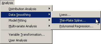
Select → → from the main menu, as shown in Figure 19.1.
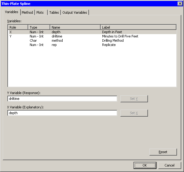
The Thin-Plate Spline dialog box appears. You can select variables for the analysis by using the Variables tab, shown in Figure 19.2. -
Select the variable
driltime, and click . -
Select the variable
depth, and click . -
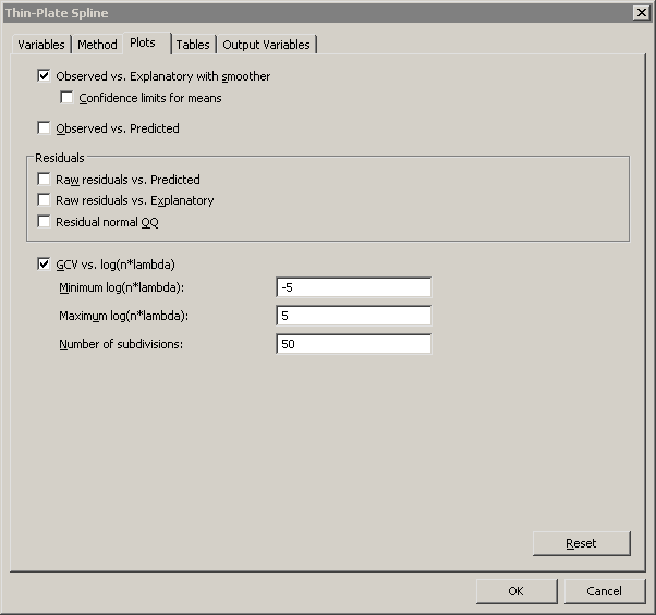
Click the Plots tab.
The Plots tab (Figure 19.3) becomes active. By default, the analysis creates a scatter plot of Y versus X with the smoother overlaid. The smoothing penalty parameter is chosen to minimize the generalized cross validation (GCV) criterion.
-
Select to visualize how the smoothing parameter affects the GCV criterion.
-
Click .
The Thin-Plate Spline analysis calls the TPSPLINE procedure with the options specified in the dialog box. The procedure displays three tables in the output document, as shown in Figure 19.4. The first table shows information about the number of observations. The second table summarizes model options used by the TPSPLINE procedure. The third table summarizes the fit, including the smoothing value (2.7433) that is chosen to optimize the selection criterion.
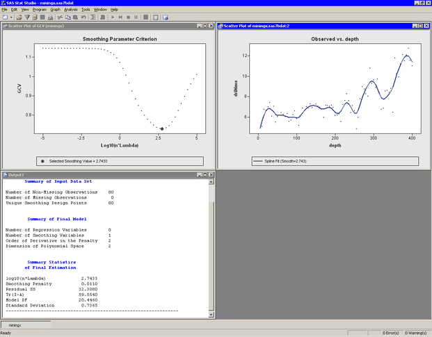
Two plots are created, as shown in Figure 19.4. The upper left plot in Figure 19.4 shows the GCV criterion for a range of smoothing parameter values. Note that the selected smoothing parameter (2.7433) is
the one that minimizes the GCV. A second plot overlays a scatter plot of driltime versus depth with a thin-plate smoother. As discussed in Chapter 18: Data Smoothing: Loess, the undulations in the smoother correspond to geological variations in the rock strata. Chapter 18: Data Smoothing: Loess, also discusses how to display multiple smoothers in a single scatter plot and how to remove smoothers from a scatter plot.