Multivariate Analysis: Canonical Discriminant Analysis

Example: Construct Linear Subspaces that Discriminate between Categories

In this example, you examine measurements of 159 fish caught in Finland’s Lake Laengelmavesi. The fish are one of seven species: bream, parkki, perch, pike, roach, smelt, and whitefish. Associated with each fish are physical measurements of weight, length, height, and width. A full description of the Fish data is included in Appendix A: Sample Data Sets.

The goal of this example is to use canonical discriminant analysis to construct linear combinations of the size and weight variables that best discriminate between the species. By looking at the coefficients of the linear combinations, you can determine which physical measurements are most important in discriminating between groups. You can also determine whether there are two or more groups that cannot be discriminated using these measurements.

To run a canonical discriminant analysis:

Open the Fish data set.
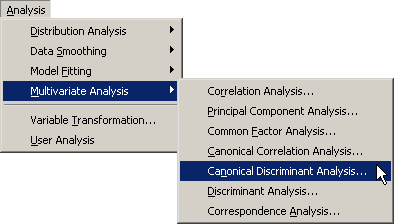
Select Analysis →Multivariate Analysis →Canonical Discriminant Analysis from the main menu, as shown in Figure 29.1.

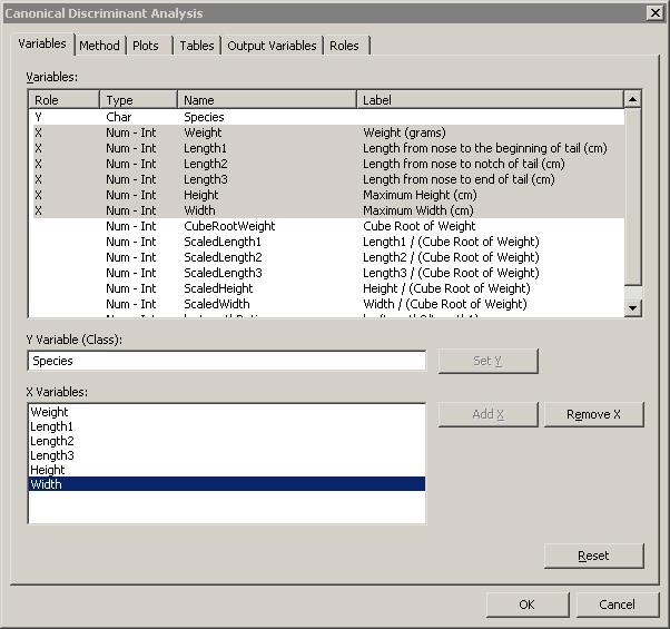
Figure 29.1: Selecting the Canonical Discriminant Analysis

The Canonical Discriminant Analysis dialog box appears. (See Figure 29.2.) You can select variables for the analysis by using the Variables tab.
Select Species and click Set Y.
Select Weight. While holding down the CTRL key, select Length1, Length2, Length3, Height, and Width. Click Add X.

Note: Alternately, you can select the variables by using contiguous selection: click the first variable (Weight), hold down the SHIFT key, and click the last variable (Width). All variables between the first and last item are selected and can be added by clicking Add X.

Figure 29.2: The Variables Tab
Click the Method tab.

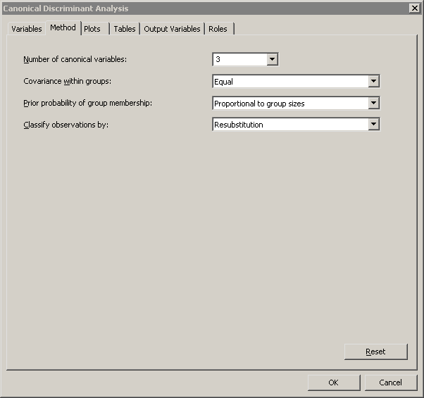
The Method tab becomes active. (See Figure 29.3.) You can use the Method tab to set options in the analysis.
Select 3 for Number of canonical variables.

The number of fish in any lake varies by species. That is, there is no reason to suspect that the number of whitefish in the lake is the same as the number of perch or bream. In the absence of prior knowledge about the distribution of fish species, you can assume that the number of fish of each species in the lake is proportional to the number in the sample.
Select Proportional to group sizes for Prior probability of group membership.

Figure 29.3: The Method Tab
Click OK.

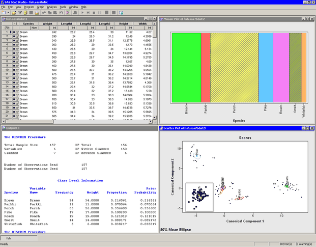
The analysis calls the DISCRIM procedure with the CANONICAL option. The procedure uses the options specified in the dialog box. The procedure displays tables in the output document, as shown in Figure 29.4. Two plots are also created.

The plot of the first two canonical components shows how well the first two canonical variables discriminate between the species of fish. The first canonical component differentiates among four groups: the pike-perch-smelt group, the roach-whitefish group, the parkki group, and the bream group. The second canonical component differentiates the pike groups from the other groups. Thus, the first two canonical components cannot differentiate between perch and smelt, nor between roach and whitefish. In Figure 29.4, a cloud of observations is selected. You can see from the linked bar chart that these observations consist of perch and smelt.

The location of the multivariate means for each species is indicated in the plot of the first two canonical components, along with an 80% confidence ellipse for the mean. The means of the perch and smelt groups are close to each other, as are the means of the roach and whitefish.

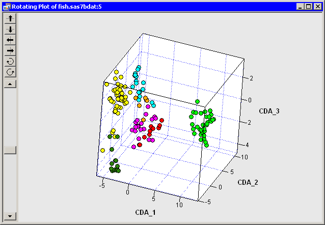
Figure 29.4: Output from a Canonical Discriminant Analysis

Note: The third canonical component helps to differentiate between perch and smelt, and between roach and whitefish. The canonical variables were added to the data table by the analysis, so you can create a scatter plot of the second and third canonical variables (CDA_3 versus CDA_2) or create a rotating plot of all three canonical components, as shown in Figure 29.5.

Figure 29.5: A Rotating Plot of the Canonical Components

The output window contains many tables of statistics. Figure 29.4 shows a summary of the model, as well as the frequency and proportion of each species.

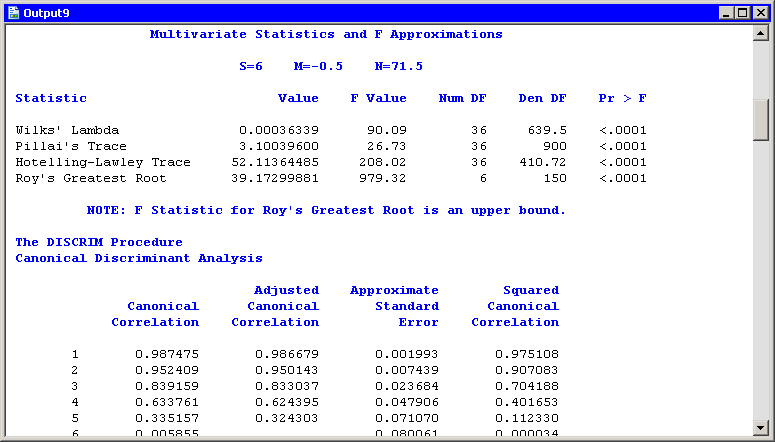
Recall that canonical discriminant analysis is equivalent to canonical correlation analysis between the quantitative variables and a set of dummy variables coded from the classification variable (in this case, Species). Figure 29.6 displays statistics that are related to the canonical correlations. The multivariate statistics and F approximations test the null hypothesis that all canonical correlations are zero. The small p-values for these tests (< 0.0001) are evidence for rejecting the null hypothesis that all canonical correlations are zero. The table of canonical correlations shows that the first three canonical components are all highly correlated with the classification variable.

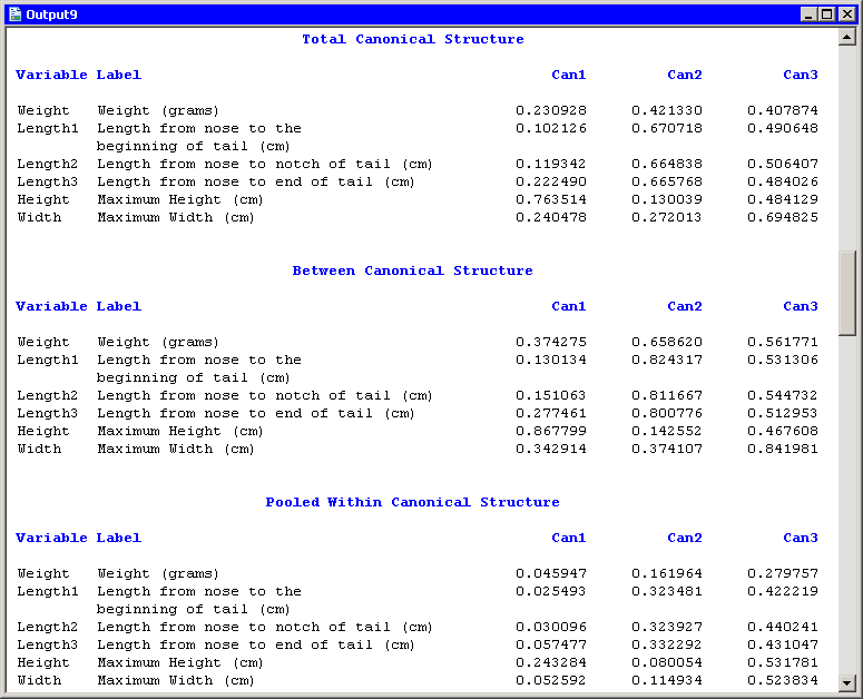
Figure 29.6: Canonical Correlations

The portion of the output window shown in Figure 29.7 shows the canonical structure. These are tables of correlations between the canonical variables and the original variables. The canonical variables are linear combinations of the original variables, so you can sometimes interpret the canonical variables in terms of the original variables.

The "Total Canonical Structure" table displays the correlations without regard for group membership. Since these correlations do not account for the groups, they can sometimes be misleading.

The "Between Canonical Structure" table removes the within-class variability before computing the correlations. For each variable X, define the group mean vector of X to be the vector whose ith element is the mean of all values of X that belong to the same group as $X_ i$ . The values in the "Between Canonical Structure" table are the correlations between the group mean vectors of the canonical variables and the group mean vectors of the original variables.

The "Pooled Within Canonical Structure" table removes the between-class variability before computing the correlations. The values in this table are the correlations between the residuals of the original and canonical variables, after regressing them onto the group variable.

For this example, the "Total Canonical Structure" table and the "Between Canonical Structure" table have similar interpretations: the first canonical component is strongly correlated with Height. The second canonical variable is strongly correlated with the length variables, and also with Weight. The third canonical component is a weighted average of all the variables, with slightly more weight given to Width.

Figure 29.7: Canonical Structure

The first canonical variable separates the species most effectively. An examination of the "Raw Canonical Coefficients" table (Figure 29.8) shows that the first canonical variable is the following linear combination of the centered variables:

$\mbox{Can}_1 = -0.0006 \: \Variable{Weight} -0.328 \: \Variable{Length1} + \ldots -1.44 \: \Variable{Width}$

The coefficients are standardized so that the canonical variables have zero mean and a pooled within-class variance equal to one.

The second canonical variable provides the greatest difference between group means while being uncorrelated with the first canonical variable.

Figure 29.8 also shows the coordinates of the group means in terms of the canonical variables. For example, the mean of the bream species projected onto the span of the first two canonical components is $(10.91, 0.51)$ . (Recall that the span of a set of vectors is the vector space consisting of all linear combinations of the vectors.) This agrees with the graph shown in Figure 29.4. The means of the perch and smelt groups are close to each other when projected onto the span of the first two canonical components. However, the third canonical component separates these means.

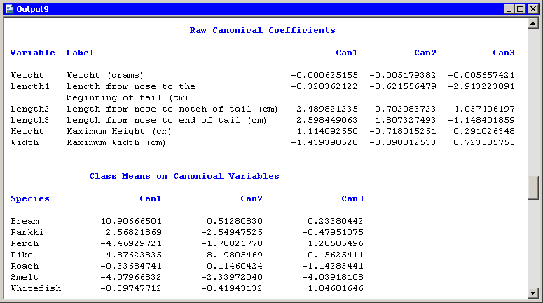
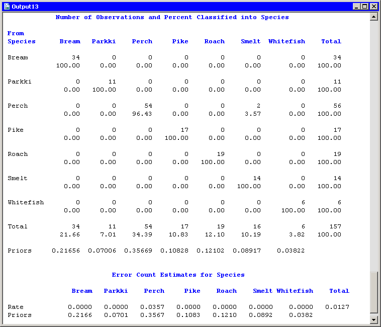
Figure 29.8: Canonical Coefficients and Group Means

Figure 29.9 displays a table that summarizes how many fish are classified (or misclassified) into each species. If the canonical components capture most of the between-class variation of the data, then the elements on the table’s main diagonal are large, compared to the off-diagonal elements. For these data, two smelt are misclassified as perch, but no other fish are misclassified. This indicates that the first three canonical components are good discriminators for Species.

Note: If you choose different options on the Method tab, the classification of observations will be different.

Figure 29.9: Classification of Observations into Groups

In summary, it is possible to use canonical discriminant analysis to discriminate between these species of fish by using three canonical components that are linear combinations of physical measurements. Trying to discriminate by using only two canonical components leads to classification errors, because the projection onto the span of the first two canonical components does not separate the perch group from the smelt group, nor does it separate the roach group from the whitefish group.