Model Fitting: Generalized Linear Models
To remove the interaction effect from the previous model and refit the data:
-
Select → → to redisplay the dialog box for this analysis.
Note: The items on the menu are not available if the output window is active. If the menu is not enabled, you should activate a graphical or tabular view of the data before clicking on the menu.
-
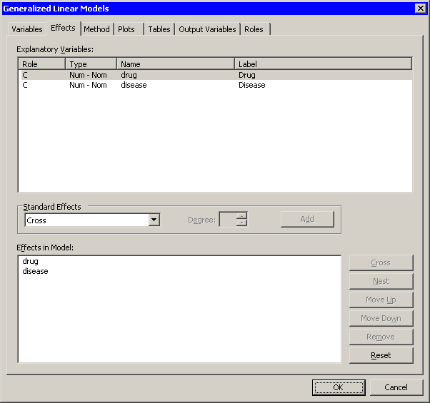
Click the Effects tab.
-
Select from the list.
-
Click .
The interaction term is removed from the list of effects, as shown in Figure 24.11.
-
Click .
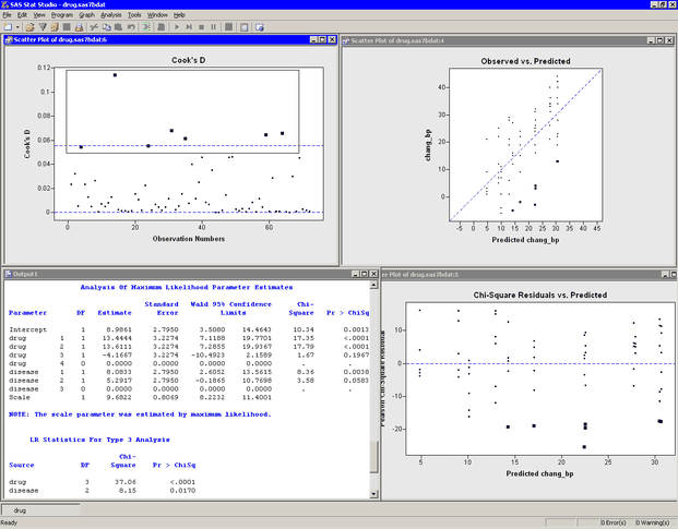
Move the workspace windows so that they are arranged as in Figure 24.12. The "LR Statistics For Type 3 Analysis" table indicates that both main effects are significant.
The "Analysis Of Maximum Likelihood Parameter Estimates" table displays parameter estimates for the model. You can use these
values to determine the predicted mean response for each experimental group. The interpretation of the parameter estimates
depends on the parameterization used to encode the classification variables in the model design matrix. This example used
the GLM coding (see Figure 24.8). For this parameterization, the predicted response for a subject is obtained by adding the estimate for the intercept to
the parameter estimates for the groups to which the subject belongs. For example, the predicted change in blood pressure in
a subject with drug=1 and disease=2 is ![]()
For a given level, the parameter estimate represents the difference between that level and the last level. For example, the estimate of the difference between the parameters for Drug 1 and Drug 4 is 13.4444, and this estimate is significantly different from zero (as indicated by the p-value in the "Pr > ChiSq" column). In contrast, the difference in the coefficients between Drug 3 and Drug 4 is –4.1667, but this estimate is not significantly different from zero. Similarly, the estimate of the difference between Disease 2 and Disease 3 is (marginally) not significant.
The parameter estimates table also estimates the scale parameter. For a normally distributed response, the scale parameter is the standard deviation of the response. See the documentation for the GENMOD procedure in the SAS/STAT User's Guide for additional details.
There are three plots in Figure 24.12. The Observed vs. Predicted plot (upper right in Figure 24.12) shows how well the model fits the data. Since this model assumes a normally distributed response with an identity link, the Chi-Square Residuals vs. Predicted plot (lower right in Figure 24.12) is just an ordinary residual plot (see the "Residuals" section of the documentation for the GENMOD procedure). The observations fall along vertical lines because all observations with the ith drug and the jth disease have the same predicted value.
The scatter plot of Cook’s D (upper left in Figure 24.12) indicates which observations have a large influence on the parameter estimates. Influential observations (that is, those with relatively large values of Cook’s D) are selected in the figure. The selected observations are highlighted in the other plots. Each observation corresponds to a large negative residual, which indicates that the observed change in blood pressure for these subjects was substantially less than the model predicts.