Example: Apply a Box-Cox Transformation :: SAS/IML(R) Studio 12.3: User's Guide

Example: Apply a Box-Cox Transformation

This example is a continuation of the previous example. The goal is the same: to normalize the driltime variable in the Miningx data set.

In the previous example, you tried a logarithmic transformation. Unfortunately, it is often not clear which transformation most improves normality. One strategy is to consider a family of transformations, and to select the transformation within the family for which the transformed data are “most normal.” The Box-Cox family (Box and Cox, 1964) is a family of power transformations that includes the logarithmic transformation as a limiting case:

$\mbox{BC}(y;\lambda ) = \left\{ \begin{array}{ll} \frac{y^\lambda - 1}{\lambda } & \mbox{if } \lambda \neq 0 \\ \log y & \mbox{if } \lambda = 0 \end{array} \right.$

The parameter $\lambda$ can be chosen by maximizing a log-likelihood function. For details see the section Normalizing Transformations.

Note: The Box-Cox parameter is traditionally denoted by $\lambda$ , as in the previous formula and in the plot in Figure 32.8. However, the Variable Transformation Wizard uses as a generic notation for a transformation parameter, as shown in Figure 32.7.

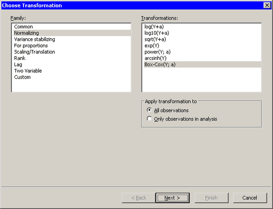
To apply a Box-Cox transformation:

Open the Miningx data set, if it is not already open.
Select Analysis →Variable Transformation from the main menu.
Select Normalizing from the Family list.
Select the Box-Cox(Y;a) transformation from the Transformations list, as shown in Figure 32.6.

Figure 32.6: Selecting a Box-Cox Transformation
Click Next.

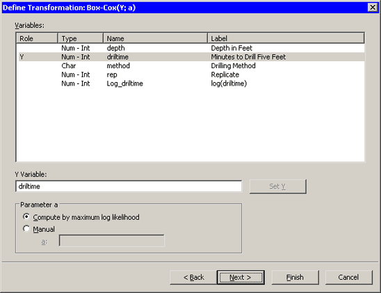
The wizard displays the page shown in Figure 32.7.

Figure 32.7: Selecting a Variable and Parameters
Select the driltime variable, and click Set Y.

By default, the Box-Cox parameter is estimated by maximum likelihood estimation. Alternatively, you can manually specify the parameter. For this example, accept the default method.

You could proceed to the next page of the wizard if you wanted to change the default name for the new variable. (The default name is BC_driltime.) For this example, accept the default name and skip the last page of the wizard.
Click Finish.

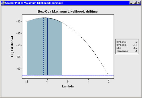
A graph appears (Figure 32.8) that plots the log-likelihood function as a function of the parameter. An inset gives the lower and upper 95% confidence limits for the maximum log-likelihood estimate, the maximum likelihood estimate (MLE), and a convenient estimate. A convenient estimate is a fraction with a small denominator (such as an integer, a half integer, or an integer multiple of or ) that is within the 95% confidence limits about the MLE. Using a convenient estimate sometimes results in a Box-Cox transformation that is more interpretable in terms of the original variable.

Note: If there is no convenient estimate within the 95% confidence limits, then the inset does not include this information.

Figure 32.8: Plot of Log Likelihood

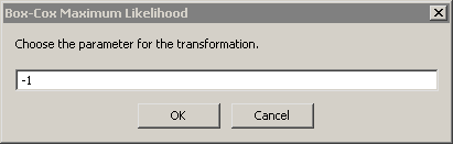
A dialog box (see Figure 32.9) also appears that prompts you for a parameter value to use for the Box-Cox transformation. For this example, you are prompted to accept the convenient estimate of –1, even though the MLE estimate is approximately –1.2.

Figure 32.9: Setting the Box-Cox Parameter
Click OK to accept the value of –1.

The parameter –1 specifies the Box-Cox transformation as 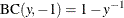$\mbox{BC}(y,-1) = 1-y^{-1}$ , which is essentially an inverse transformation followed by a reflection and translation.

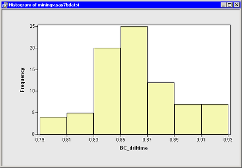
To complete this example, you can visualize the distribution of the new variable.
Create a histogram of the BC_driltime variable.

The histogram is shown in Figure 32.10. The transformed data show improved normality: the distribution is more symmetric and the tails are not as long.

Figure 32.10: Histogram of the Box-Cox Transformed Data