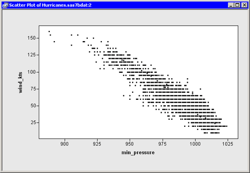
In this example, you create a polynomial regression analysis of wind_kts as a function of min_pressure in the Hurricanes data set. The wind_kts variable is the wind speed in knots; the min_pressure variable is the minimum central pressure for each observation.
A scatter plot of these variables indicates that the relationship between these variables is approximately linear, as shown in Figure 20.1, so this example fits a line to the data.
To create a polynomial regression analysis:
-
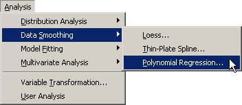
Select → → from the main menu, as shown in Figure 20.2.
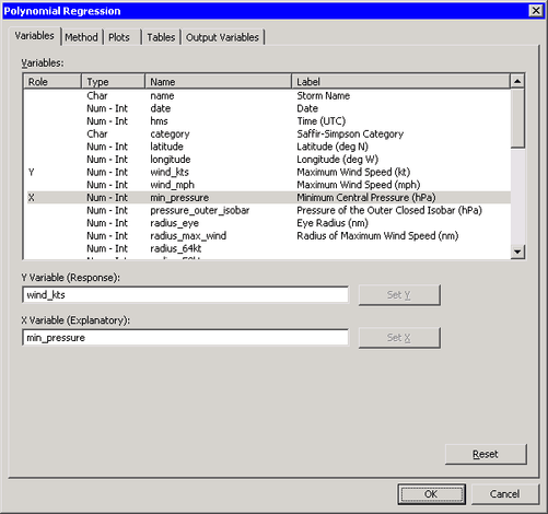
The Polynomial Regression dialog box appears. (See Figure 20.3.)
-
Select the variable
wind_kts, and click . -
Select the variable
min_pressure, and click . -
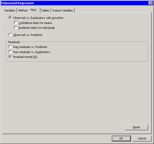
Click the Plots tab.
The Plots tab becomes active. This tab controls which graphs are produced by the analysis, and the options for each graph (for example, whether to display confidence limits).
By default, the analysis creates a scatter plot of the observed X and Y variables, with a smoother added. You can decide whether or not to plot confidence limits.
-
Clear .
-
Select .
-
Click .
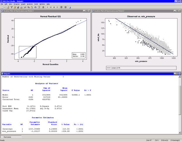
Several plots appear, along with output from the REG procedure. (See Figure 20.5.) A scatter plot shows the bivariate data and the requested linear smoother. The analysis also creates a normal Q-Q plot of the residuals. The Q-Q plot indicates that quite a few observations have wind speeds that are substantially lower than would be expected by assuming a linear model with normally distributed errors. In Figure 20.5 these observations are selected, and the corresponding markers in the scatter plot are highlighted.
Output from the REG procedure appears in the output document. The output informs you that
min_pressurehas three missing values; those observations are not included in the analysis. The parameter estimates table indicates that when the central atmospheric pressure of a cyclone decreases by 1 hPa, you can expect the wind speed to increase by about 1.3 knots.