Graphical Layouts

One of most powerful features of the GTL is the syntax built around hierarchical statement blocks called “layouts.” The outermost layout block determines

The overall organization of the graph—whether it uses a single-cell or a multi-cell display.
What statements are allowed in the block. Generally, layout blocks can contain plots, lines of text, a legend, or even another layout.
How the contained statements interact.

Outermost Layouts in GTL

Layout	Description
OVERLAY	General purpose layout for displaying 2-D plots in a single-cell.
OVERLAY3D	Layout for displaying 3-D plots in a single-cell.
OVERLAYEQUATED	Specialized OVERLAY with equated axes.
GRIDDED	Basic grid of plots. All cells are independent.
LATTICE	Advanced multi-cell layout. Axes can be shared across columns or rows and be external to grid. Many grid labeling and alignment features.
DATALATTICE	Generates a classification panel from the values of 1 or 2 classifiers.
DATAPANEL	Generates a classification panel from the values of n classifiers.

For example, the following graph is a two-cell graph produced using the LAYOUT LATTICE statement as the outermost template in the layout.

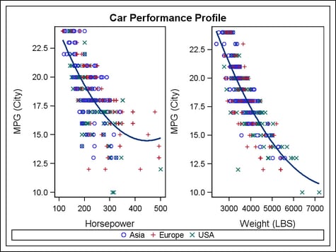
The LAYOUT LATTICE statement is typically used to create a multi-cell layout of plots that are aligned across columns and rows. In the following template, which produced the graph, plot statements are specified within nested LAYOUT OVERLAY statements. Thus, the LATTICE automatically aligns the plot areas and tick display areas in the plots. The LATTICE layout is a good layout to choose when you want to compare the results of related plots.

proc template;
  define statgraph lattice;
  begingraph;
    entrytitle "Car Performance Profile";
    layout lattice / border=true pad=10 opaque=true
                     rows=1 columns=2 columngutter=3;
      layout overlay;
        scatterplot x=horsepower y=mpg_city /
          group=origin name="cars";
        regressionPlot x=horsepower y=mpg_city / degree=2;
      endlayout;

      layout overlay;
        scatterplot x=weight y=mpg_city / group=origin;
        regressionPlot x=weight y=mpg_city / degree=2;
      endlayout;
      
      sidebar;
        discretelegend "cars";
      endsidebar;
    endlayout;
  endgraph;
  end;
run;

For detailed information about each layout, see the chapter for that layout type.