Forecasting Process Details
Intervention Effects
Interventions are used for modeling events that occur at specific times. That is, they are known changes that affect the dependent series or outliers.
The ith intervention series is included in the output data set with variable name _INTVi _, which is a reserved variable name.
Point Interventions
The point intervention is a one-time event. The ith intervention series  has a point intervention at time
  when the series is nonzero only at time —that is,
![\[ X_{i,t} = \begin{cases} 1,& t = t_{int} \\ 0,& otherwise \end{cases} \]](images/etsug_tffordet0188.png)
Step Interventions
Step interventions are continuing, and the input time series flags periods after the intervention. For a step intervention,
before time , the ith intervention series is zero and then steps to a constant level thereafter—that is,
![\[ X_{i,t} = \begin{cases} 1,& t \ge t_{int} \\ 0,& otherwise \end{cases} \]](images/etsug_tffordet0189.png)
Ramp Interventions
A ramp intervention is a continuing intervention that increases linearly after the intervention time. For a ramp intervention,
before time , the ith intervention series  is zero and increases linearly thereafter—that is, proportional to time.
![\[ X_{i,t} = \begin{cases} t - t_{int},& t \ge t_{int} \\ 0,& otherwise \end{cases} \]](images/etsug_tffordet0191.png)
Intervention Effect
Given the ith intervention series , you can define how the intervention takes effect by filters (transfer functions) of the form
![\[ {\Psi }_{i}({B})=\frac{1-{\omega }_{i,1}{B}-{\ldots }- {\omega }_{i,q_{i}}{B}^{q_{i}}}{1-{\delta }_{i,1}{B}-{\ldots }- {\delta }_{i,p_{i}}{B}^{p_{i}}} \]](images/etsug_tffordet0192.png)
where  is the backshift operator
  .
.
The denominator of the transfer function determines the decay pattern of the intervention effect, whereas the numerator terms determine the size of the intervention effect time window.
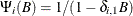
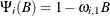
For example, the following intervention effects are associated with the respective transfer functions.
-
- Immediately
-

- Gradually
-
- 1 lag window
-
- 3 lag window
-

Intervention Notation
The notation used to describe intervention effects has the form type :t (q
(q )/(p), where type is point, step, or ramp; t is the time of the intervention (for example, OCT87); q is the transfer function numerator order; and p is the transfer function denominator order. If
  , the part "(q)" is omitted; if
  , the part "/(p)" is omitted.
In the Intervention Specification window, the Number of Lags option specifies the transfer function numerator order q, and the Effect Decay Pattern option specifies the transfer function denominator order p. In the Effect Decay Pattern options, values and resulting p are: None, ; Exp,  ;
; Wave,  .
.
For example, a step intervention with date 08MAR90 and effect pattern Exp is denoted "Step:08MAR90/(1)" and has a transfer function filter 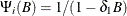 . A ramp intervention immediately applied on 08MAR90 is denoted "Ramp:08MAR90" and has a transfer function filter .