The MODEL Procedure

Example 26.22 Reducing Parameter Variance in a Tree Biomass Model

This example uses various dimensions of willow oak trees to model their biomass. Unlike a tree’s biomass, a tree’s dimensions can be measured noninvasively. The model and data for this example are taken from Parresol (1999). This biomass model uses four equations to model the bole wood, bole bark, crown, and total mass of the trees,

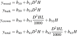
$\begin{align*} y_\text {wood} & = b_{10} + b_{11}D^2H \\ y_\text {bark} & = b_{20} + b_{21}D^2H \\ y_\text {crown} & = b_{30} + b_{31}\frac{D^2H L}{1000} + b_{32}H \\ y_\text {total} & = b_{40} + b_{41}D^2H + b_{42}\frac{D^2H L}{1000} + b_{43}H \end{align*}$

where $y_\text {wood}$ , $y_\text {bark}$ , and $y_\text {crown}$ are the three components of a tree’s total biomass, $y_\text {total}$ ; D is the tree’s diameter at breast height; H is the tree’s height; and L is the tree’s live crown length. The efficiency of parameter estimates in this model is improved by taking into account the correlations between errors in the equations for the four components of the trees’ biomass. Also, the efficiency of estimates is improved by taking into account heteroscedasticity in the sample of 39 trees that is used to develop the model.

In an initial OLS estimation of this model’s parameters, some general properties of the model and data can be quantified using the following statements:

proc model data=trees;
   endo wood bark crown total;

   vol = dbh**2*height;
   cvol = vol*lcl/1000;

   wood  = b10 + b11*vol;
   bark  = b20 + b21*vol;
   crown = b30 + b31*cvol + b32*height;
   total = b40 + b41*vol + b42*cvol + b43*height;

   fit / ols outs=stree out=otree outresid;
quit;

Here the covariance of equation errors is saved to the data set STREE, and the residuals are saved to the data set OTREE for later analysis.

The covariance matrix of equation errors that is computed in the OLS estimation can be used in a seemingly unrelated regression (SUR) estimation of the model to improve the efficiency of parameter estimates. The total biomass of trees is restricted to equal the other three biomass components in the following SUR estimation:

proc model data=trees;
   endo wood bark crown total;

   vol = dbh**2*height;
   cvol = vol*lcl/1000;

   wood  = b10 + b11*vol;
   bark  = b20 + b21*vol;
   crown = b30 + b31*cvol + b32*height;
   total = b40 + b41*vol + b42*cvol + b43*height;

   fit / nools sur sdata=stree;

   restrict b10 + b20 + b30 = b40,
            b11 + b21 = b41,
            b42 = b31,
            b43 = b32;
quit;

Output 26.22.1 shows the parameters and standard errors for the restricted SUR tree biomass model.

Output 26.22.1: SUR Parameter Estimates for Willow Oak Model

The MODEL Procedure

Nonlinear SUR Parameter Estimates
Parameter	Estimate	Approx Std Err	t Value	Approx Pr > \|t\|	Label
b10	59.18653	48.2435	1.23	0.2274
b11	0.026598	0.000558	47.67	<.0001
b20	29.65101	10.3839	2.86	0.0069
b21	0.003225	0.000120	26.79	<.0001
b30	133.1066	26.6246	5.00	<.0001
b31	0.061543	0.00508	12.11	<.0001
b32	-5.33604	1.1141	-4.79	<.0001
b40	221.9441	62.1834	3.57	0.0010
b41	0.029824	0.000623	47.91	<.0001
b42	0.061543	0.00508	12.11	<.0001
b43	-5.33604	1.1141	-4.79	<.0001
Restrict0	-656E-14	0.1316	-0.00	1.0000	b10 + b20 + b30 = b40
Restrict1	148.5607	11355.0	0.01	0.9898	b11 + b21 = b41
Restrict2	68.66564	178.8	0.38	0.7067	b42 = b31
Restrict3	0.388714	3.5449	0.11	0.9145	b43 = b32

An analysis of heteroscedasticity in the unrestricted OLS model suggests that the efficiency of the estimation could be improved further by weighting the observations using the following variance model:

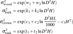
$\begin{align*} \sigma ^2_\text {wood} & = \exp (w_1 + w_2\ln D^2 H) \\ \sigma ^2_\text {bark} & = \exp (k_1 + k_2\ln D^2 H) \\ \sigma ^2_\text {crown} & = \exp (c_1 + c_2\ln \frac{D^2H L}{1000} - c_3 H^2) \\ \sigma ^2_\text {total} & = \exp (t_1 + t_2\ln D^2 H) \end{align*}$

where $\sigma ^2_ i$ is the variance of the ith component of the biomass and the parameters $w_1$ , $w_2$ , $k_1$ , $k_2$ , $c_1$ , $c_2$ , $c_3$ , $t_1$ , and $t_2$ are determined by regressing the square of the residuals from the unrestricted OLS estimation against the tree dimensions. Estimates of the parameters in the variance model can be determined using the following statements:

proc model data=otree;
   vol = dbh**2*height;
   cvol = vol*lcl/1000;

   eq.varwood  = log(wood*wood) - (w1 + w2*log(vol));
   eq.varbark  = log(bark*bark) - (k1 + k2*log(vol));
   eq.varcrown = log(crown*crown) - (c1 + c2*log(cvol) - c3*height**2);
   eq.vartotal = log(total*total) - (t1 + t2*log(vol));

   fit varwood varbark varcrown vartotal;
quit;

The biomass component variance model can be used to account for heteroscedasticity and improve the efficiency of parameter estimates by weighting observations in the biomass model. The following PROC MODEL statements accommodate both the covariance among the biomass equations’ errors and the heteroscedasticity that is observed in each component of the trees’ biomass:

proc model data=trees;
   endo wood bark crown total;

   vol = dbh**2*height;
   cvol = vol*lcl/1000;

   wood  = b10 + b11*vol;
   bark  = b20 + b21*vol;
   crown = b30 + b31*cvol + b32*height;
   total = b40 + b41*vol + b42*cvol + b43*height;

   h.wood = exp(&w1)*vol**&w2;
   h.bark = exp(&k1)*vol**&k2;
   h.crown = exp(&c1)*cvol**&c2 * exp (-&c3*height*height);
   h.total = exp(&t1)*vol**&t2;

   fit / sur;

   restrict b10 + b20 + b30 = b40,
            b11 + b21 = b41,
            b42 = b31,
            b43 = b32;
quit;

Output 26.22.2 shows the parameters and standard errors for the heteroscedastic tree biomass model.

Output 26.22.2: SUR Parameter Estimates for Heteroscedastic Willow Oak Model

The MODEL Procedure

Nonlinear SUR Parameter Estimates
Parameter	Estimate	Approx Std Err	t Value	Approx Pr > \|t\|	Label
b10	10.22253	14.2208	0.72	0.4766
b11	0.027515	0.000534	51.48	<.0001
b20	15.66358	4.8173	3.25	0.0024
b21	0.003476	0.000138	25.13	<.0001
b30	103.8782	10.6122	9.79	<.0001
b31	0.055226	0.00306	18.02	<.0001
b32	-4.05163	0.4603	-8.80	<.0001
b40	129.7643	21.5621	6.02	<.0001
b41	0.030991	0.000614	50.47	<.0001
b42	0.055226	0.00306	18.02	<.0001
b43	-4.05163	0.4603	-8.80	<.0001
Restrict0	-0.28369	1.1969	-0.24	0.8164	b10 + b20 + b30 = b40
Restrict1	-56046.2	49194.0	-1.14	0.2603	b11 + b21 = b41
Restrict2	539.3854	697.4	0.77	0.4471	b42 = b31
Restrict3	4.374001	29.6959	0.15	0.8853	b43 = b32

Output 26.22.3 shows the improved efficiency of estimates in the heteroscedastic model as compared to the homoscedastic model. For most of the parameters, the standard errors are reduced significantly in the heteroscedastic estimation.

Output 26.22.3: Standard Error Reduction

Parameter	StdErr Rel. Change
b10	( 71%)
b11	( 4%)
b20	( 54%)
b21	15%
b30	( 60%)
b31	( 40%)
b32	( 59%)
b40	( 65%)
b41	( 1%)
b42	( 40%)
b43	( 59%)