Example 19.12 Cauchy Distribution Estimation :: SAS/ETS(R) 12.3 User's Guide

Example 19.12 Cauchy Distribution Estimation

In this example a nonlinear model is estimated by using the Cauchy distribution. Then a simulation is done for one observation in the data.

The following DATA step creates the data for the model.

/* Generate a Cauchy distributed Y */
data c;
   format date monyy.;
   call streaminit(156789);
   do t=0 to 20 by 0.1;
      date=intnx('month','01jun90'd,(t*10)-1);
      x=rand('normal');
      e=rand('cauchy') + 10 ;
      y=exp(4*x)+e;
      output;
   end;
run;

The model to be estimated is

$\displaystyle y$	$\displaystyle =$	$\displaystyle e^{-a~ x} + \epsilon$
$\displaystyle \epsilon$	$\displaystyle \sim$	$\displaystyle \textrm{Cauchy} ( nc )$

That is, the residuals of the model are distributed as a Cauchy distribution with noncentrality parameter .

The log likelihood for the Cauchy distribution is

$\textrm{ll} = -\log \pi (1+(x-nc)^2)$

The following SAS statements specify the model and the log-likelihood function.

title1 'Cauchy Distribution';

proc model data=c ;
   dependent y;
   parm a -2 nc 4;
   y=exp(-a*x);

       /* Likelihood function for the residuals */
   obj = log(constant('pi')*(1+(-resid.y-nc)**2));

   errormodel y ~ general(obj) cdf=cauchy(nc);

   fit y / outsn=s1 method=marquardt;
   solve y / sdata=s1 data=c(obs=1) random=1000
             seed=256789 out=out1;
run;

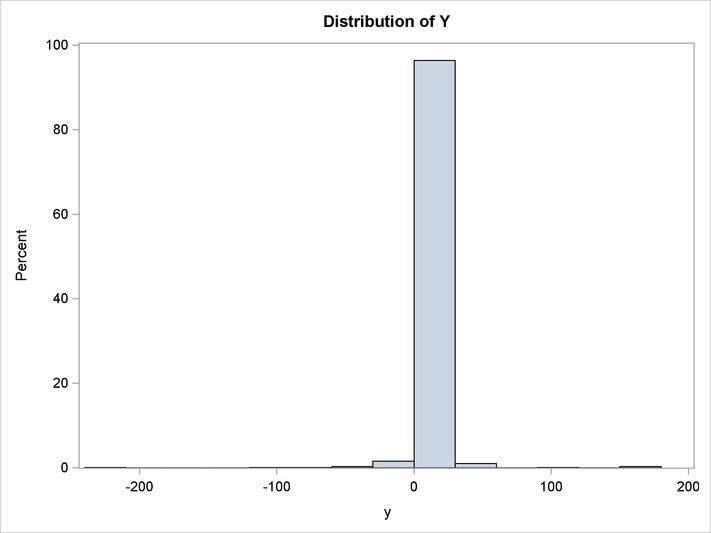
title 'Distribution of Y';
proc sgplot data=out1;
   histogram y;
run;

The FIT statement uses the OUTSN= option to output the $\bSigma$ matrix for residuals from the normal distribution. The $\bSigma$ matrix is $1\times 1$ and has value because it is a correlation matrix. The OUTS= matrix is the scalar . Because the distribution is univariate (no covariances), the OUTS= option would produce the same simulation results. The simulation is performed by using the SOLVE statement.

The distribution of is shown in the following output.

Output 19.12.1: Distribution of Y