Window Reference

Time Series Viewer Window

Use the Time Series Viewer window to explore time series data using plots, transformations, statistical tests, and tables. It is available as a standalone application and as part of the Time Series Forecasting System. To use it as a standalone application, select it from the Analysis submenu of the Solutions menu, or use the tsview command (see Chapter 44, Command Reference, in this book). To use it within the Time Series Forecasting System, select the View Series Graphically icon in the Time Series Forecasting, Develop Models, or Model List window, or select "Series" from the View menu of the Develop Models, Manage Project, or Model List window.

The various plots and tables available are referred to as views. The section View Selection Icons explains how to change the view.

The state of the Time Series Viewer window is controlled by the current series, the current series transformation specification, and the currently selected view. You can resize this window, and you can use other windows without closing the Time Series Viewer window. You can explore a number of series conveniently by keeping the Series Selection window open. Each time you make a selection, the viewer window is updated to show the selected series. Keep both windows visible, or switch between them by using the Next Viewer toolbar icon or the F12 function key.

You can open multiple Time Series Viewer windows. This enables you to “freeze”a plot so you can come back to it later, or compare two plots side by side on your screen. To do this, unlink the viewer by using the Link/Unlink icon on the window’s toolbar or the corresponding item in the Tools menu. While the viewer window remains unlinked, it is not updated when other selections are made in the Series Selection window. Instead, when you select a series and click the Graph button, a new Time Series Viewer window is invoked. You can continue this process to open as many viewer windows as you want. The Next Viewer icon and corresponding F12 function key are useful for navigating between windows when they are not simultaneously visible on your screen.

A wide range of series transformations is available. Basic transformations are available from the window’s horizontal toolbar, and others are available by selecting "Other Transformations" from the Tools menu.

Horizontal Tool Bar

The Time Series Viewer window contains a horizontal toolbar with the following icons:

Zoom in: changes the mouse cursor into cross hairs that you can use with the left mouse button to drag out a region of the time series plot to zoom in on. In the Autocorrelations view and the White Noise and Stationarity Tests view, Zoom In reduces the number of lags displayed.
Zoom out: reverses the previous Zoom In action and expands the time range of the plot to show more of the series. In the Autocorrelations view and the White Noise and Stationarity Tests view, Zoom Out increases the number of lags displayed.
Link/Unlink viewer: disconnects or connects the Time Series Viewer window to the window in which the series was selected. When the Viewer is linked, it always shows the current series. If you select another series, linked Viewers are updated. Unlinking a Viewer freezes its current state, and changing the current series has no effect on the Viewer’s display. The View Series action creates a new Series Viewer window if there is no linked Viewer. By using the unlink feature, you can open several Time Series Viewer windows and display several different series simultaneously.
Log Transform: applies a log transform to the current view. This can be combined with other transformations; the current transformations are shown in the title.
Difference: applies a simple difference to the current view. This can be combined with other transformations; the current transformations are shown in the title.
Seasonal Difference: applies a seasonal difference to the current view. For example, if the data are monthly, the seasonal cycle is one year. Each value has subtracted from it the value from one year previous. This can be combined with other transformations; the current transformations are shown in the title.
Close: closes the Time Series Viewer window and returns to the window from which it was invoked.

Vertical Toolbar View Selection Icons

At the right-hand side of the Time Series Viewer window is a vertical toolbar used to select the kind of plot or table that the Viewer displays.

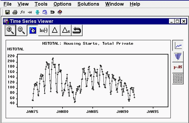
Series

displays a plot of series values over time.

Autocorrelations

displays plots of the sample autocorrelations, partial autocorrelation, and inverse autocorrelation functions for the series, with lines overlaid at plus and minus two standard errors.

White Noise and Stationarity Tests

displays horizontal bar charts that represent results of white noise and stationarity tests. The first bar chart shows the significance probability of the Ljung-Box chi-square statistic computed on autocorrelations up to the given lag. Longer bars favor rejection of the null hypothesis that the series is white noise. Click any of the bars to display an interpretation.

The second bar chart shows tests of stationarity, where longer bars favor the conclusion that the series is stationary. Each bar displays the significance probability of the augmented Dickey-Fuller unit root test to the given autoregressive lag. Long bars represent higher levels of significance against the null hypothesis that the series contains a unit root. For seasonal data, a third bar chart appears for seasonal root tests. Click any of the bars to display an interpretation.

Data Table

displays a data table containing the values in the input data set.

Menu Bar

File

Save Graph: saves the current plot as a SAS/GRAPH grseg catalog entry in a default or most recently specified catalog. This item is unavailable in the Data Table view.
Save Graph as: saves the current graph as a SAS/GRAPH grseg catalog entry in a SAS catalog that you specify and/or as an Output Delivery System (ODS) object. By default, an HTML page is created, with the graph embedded as a gif image. This item is unavailable in the Data Table view.
Save Data: saves the data displayed in the viewer window to an output SAS data set. This item is unavailable in the Series view.
Save Data as: saves the data in a SAS data set that you specify and/or as an Output Delivery System (ODS) object. By default, an HTML page is created, with the data displayed as a table.
Import Data: is available if you license SAS/Access software. It opens an Import Wizard, which you can use to import your data from an external spreadsheet or data base to a SAS data set for use in the Time Series Forecasting System.
Export Data: is available if you license SAS/Access software. It opens an Export Wizard, which you can use to export a SAS data set, such as a forecast data set created with the Time Series Forecasting System, to an external spreadsheet or data base.
Print Graph: prints the plot displayed in the viewer window. This item is unavailable in the Data Table view.
Print Data: prints the data displayed in the viewer window. This item is unavailable in the Series view.
Print Setup: opens the Print Setup window, which allows you to access your operating system print setup.
Print Preview: opens a preview window to show how your plots will look when printed.
Close: closes the Time Series Viewer window and returns to the window from which it was invoked.

View

Series: displays a plot of series values over time. This is the same as the Series icon in the vertical toolbar.
Autocorrelations: displays plots of the sample autocorrelation, partial autocorrelation, and inverse autocorrelation functions for the series. This is the same as the Autocorrelations icon in the vertical toolbar.
White Noise and Stationarity Tests: displays horizontal bar charts representing results of white noise and stationarity tests. This is the same as the White Noise and Stationarity Tests icon in the vertical toolbar.
Data Table: displays a data table containing the values in the input data set. This is the same as the Data Table icon in the vertical toolbar.
Zoom In: zooms the display. This is the same as the Zoom In icon in the window’s horizontal toolbar.
Zoom Out: undoes the last zoom in action. This is the same as the Zoom Out icon in the window’s horizontal toolbar.
Zoom Way Out: reverses all previous Zoom In actions and expands the time range of the plot to show all of the series, or shows the maximum number of lags in the Autocorrelations View or the White Noise and Stationarity Tests view.

Tools

Log Transform: applies a log transformation. This is the same as the Log Transform icon in the window’s horizontal toolbar.
Difference: applies simple differencing. This is the same as the Difference icon in the window’s horizontal toolbar.
Seasonal Difference: applies seasonal differencing. This is the same as the Seasonal Difference icon in the window’s horizontal toolbar.
Other Transformations: opens the Series Viewer Transformations window to enable you to apply a wide range of transformations.
Diagnose Series: opens the Series Diagnostics window to determine the kinds of forecasting models appropriate for the current series.
Define Interventions: opens the Interventions for Series window to enable you to edit or add intervention effects for use in modeling the current series.
Link Viewer: connects or disconnects the Time Series Viewer window to the window from which series are selected. This is the same as the Link item in the window’s horizontal toolbar.

Options

Number of Lags: opens a window to let you specify the number of lags shown in the Autocorrelations view and the White Noise and Stationarity Tests view. You can also use the Zoom In and Zoom Out actions to control the number of lags displayed.
Correlation Probabilities: controls whether the bar charts in the Autocorrelations view represent significance probabilities or values of the correlation coefficient. A check mark or filled check box next to this item indicates that significance probabilities are displayed. In each case the bar graph horizontal axis label changes accordingly.

Mouse Button Actions

You can examine the data value and date of individual points in the Series view by clicking them. The date and value are displayed in a box that appears in the upper right corner of the Viewer window. Click the mouse elsewhere or select any action to dismiss the data box.

You can examine the values of the bars and confidence limits at different lags in the Autocorrelations view by clicking individual bars in the vertical bar charts.

You can display an interpretation of the tests in the White Noise and Stationarity Tests view by clicking the bars.

When you select the Zoom In action, you can use the mouse to define a region of the graph to take a closer look at. Position the mouse cursor at one corner of the region, press the left mouse button, and move the mouse cursor to the opposite corner of the region while holding the left mouse button down. When you release the mouse button, the plot is redrawn to show an expanded view of the data within the region you selected.

Top of Page