Forecasting Process Details :: SAS/ETS(R) 9.22 User's Guide

Forecasting Process Details

Notation for ARIMA Models

A dependent time series that is modeled as a linear combination of its own past values and past values of an error series is known as a (pure) ARIMA model.

Nonseasonal ARIMA Model Notation

The order of an ARIMA model is usually denoted by the notation ARIMA(p,d,q), where

p: is the order of the autoregressive part.
d: is the order of the differencing (rarely should $\text{[math]}$ > 2 be needed).
q: is the order of the moving-average process.

Given a dependent time series $\text{[math]}$ , mathematically the ARIMA model is written as

$\text{[math]}$

where

t: indexes time.
$\text{[math]}$: is the mean term.
$\text{[math]}$: is the backshift operator; that is, $\text{[math]}$ .
$\text{[math]}$: is the autoregressive operator, represented as a polynomial in the back shift operator: $\text{[math]}$ .
$\text{[math]}$: is the moving-average operator, represented as a polynomial in the back shift operator: $\text{[math]}$ .
$\text{[math]}$: is the independent disturbance, also called the random error.

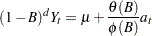
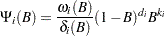
For example, the mathematical form of the ARIMA(1,1,2) model is

$\text{[math]}$

Seasonal ARIMA Model Notation

Seasonal ARIMA models are expressed in factored form by the notation ARIMA(p,d,q)(P,D,Q) $\text{[math]}$ , where

P: is the order of the seasonal autoregressive part.
D: is the order of the seasonal differencing (rarely should D > 1 be needed).
Q: is the order of the seasonal moving-average process.
s: is the length of the seasonal cycle.

Given a dependent time series $\text{[math]}$ , mathematically the ARIMA seasonal model is written as

$\text{[math]}$

where

$\text{[math]}$: is the seasonal autoregressive operator, represented as a polynomial in the back shift operator:
$\text{[math]}$
$\text{[math]}$: is the seasonal moving-average operator, represented as a polynomial in the back shift operator: $\text{[math]}$

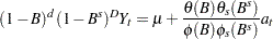
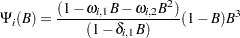
For example, the mathematical form of the ARIMA(1,0,1)(1,1,2) $\text{[math]}$ model is

$\text{[math]}$

Abbreviated Notation for ARIMA Models

If the differencing order, autoregressive order, or moving-average order is zero, the notation is further abbreviated as

I(d)(D) $\text{[math]}$: integrated model or ARIMA(0,d,0)(0,D,0)
AR(p)(P) $\text{[math]}$: autoregressive model or ARIMA(p,0,0)(P,0,0)
IAR(p,d)(P,D) $\text{[math]}$: integrated autoregressive model or ARIMA(p,d,0)(P,D,0) $\text{[math]}$
MA(q)(Q) $\text{[math]}$: moving average model or ARIMA(0,0,q)(0,0,Q) $\text{[math]}$
IMA(d,q)(D,Q) $\text{[math]}$: integrated moving average model or ARIMA(0,d,q)(0,D,Q) $\text{[math]}$
ARMA(p,q)(P,Q) $\text{[math]}$: autoregressive moving-average model or ARIMA(p,0,q)(P,0,Q) $\text{[math]}$ .

Notation for Transfer Functions

A transfer function can be used to filter a predictor time series to form a dynamic regression model.

Let $\text{[math]}$ be the dependent series, let $\text{[math]}$ be the predictor series, and let $\text{[math]}$ be a linear filter or transfer function for the effect of $\text{[math]}$ on $\text{[math]}$ . The ARIMA model is then

$\text{[math]}$

This model is called a dynamic regression of $\text{[math]}$ on $\text{[math]}$ .

Nonseasonal Transfer Function Notation

Given the ith predictor time series $\text{[math]}$ , the transfer function is written as

$\text{[math]}$

where

d $\text{[math]}$: is the simple order of the differencing for the ith predictor time series, $\text{[math]}$ (rarely should $\text{[math]}$ > 2 be needed).
k $\text{[math]}$: is the pure time delay (lag) for the effect of the ith predictor time series, $\text{[math]}$ .
p $\text{[math]}$: is the simple order of the denominator for the ith predictor time series.
q $\text{[math]}$: is the simple order of the numerator for the ith predictor time series.

The mathematical notation used to describe a transfer function is

$\text{[math]}$

where

$\text{[math]}$: is the backshift operator; that is, $\text{[math]}$ .
$\text{[math]}$: is the denominator polynomial of the transfer function for the ith predictor time series: $\text{[math]}$ .
$\text{[math]}$: is the numerator polynomial of the transfer function for the ith predictor time series: $\text{[math]}$ .

The numerator factors for a transfer function for a predictor series are like the MA part of the ARMA model for the noise series. The denominator factors for a transfer function for a predictor series are like the AR part of the ARMA model for the noise series. Denominator factors introduce exponentially weighted, infinite distributed lags into the transfer function.

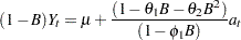
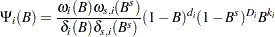
For example, the transfer function for the ith predictor time series with

$\text{[math]}$: time lag is 3
$\text{[math]}$: simple order of differencing is one
$\text{[math]}$: simple order of the denominator is one
$\text{[math]}$: simple order of the numerator is two

would be written as [Dif(1)Lag(3)N(2)/D(1)]. The mathematical notation for the transfer function in this example is

$\text{[math]}$

Seasonal Transfer Function Notation

The general transfer function notation for the ith predictor time series X $\text{[math]}$ with seasonal factors is [Dif(d $\text{[math]}$ )(D $\text{[math]}$ ) $\text{[math]}$ Lag(k $\text{[math]}$ ) N(q $\text{[math]}$ )(Q $\text{[math]}$ ) $\text{[math]}$ / D(p $\text{[math]}$ )(P $\text{[math]}$ ) $\text{[math]}$ ] where

D $\text{[math]}$: is the seasonal order of the differencing for the ith predictor time series (rarely should D $\text{[math]}$ > 1 be needed).
P $\text{[math]}$: is the seasonal order of the denominator for the ith predictor time series (rarely should P $\text{[math]}$ > 2 be needed).
Q $\text{[math]}$: is the seasonal order of the numerator for the ith predictor time series, (rarely should Q $\text{[math]}$ > 2 be needed).
s: is the length of the seasonal cycle.

The mathematical notation used to describe a seasonal transfer function is

$\text{[math]}$

where

$\text{[math]}$: is the denominator seasonal polynomial of the transfer function for the ith predictor time series:
$\text{[math]}$
$\text{[math]}$: is the numerator seasonal polynomial of the transfer function for the ith predictor time series:
$\text{[math]}$

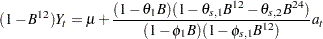
For example, the transfer function for the ith predictor time series X $\text{[math]}$ whose seasonal cycle $\text{[math]}$ with

$\text{[math]}$: simple order of differencing is two
$\text{[math]}$: seasonal order of differencing is one
$\text{[math]}$: simple order of the numerator is two
$\text{[math]}$: seasonal order of the numerator is one

would be written as [Dif(2)(1) $\text{[math]}$ N(2)(1) $\text{[math]}$ ]. The mathematical notation for the transfer function in this example is

$\text{[math]}$

Note: In this case, [Dif(2)(1) $\text{[math]}$ N(2)(1) $\text{[math]}$ ] = [Dif(2)(1) $\text{[math]}$ Lag(0)N(2)(1) $\text{[math]}$ /D(0)(0) $\text{[math]}$ ].

Top of Page