PROC MODEL: Mixtures of Distributions—Copulas :: SAS/ETS(R) 9.22 User's Guide

The MODEL Procedure

Mixtures of Distributions—Copulas

The theory of copulas is what enables the MODEL procedure to combine and simulate multivariate distributions with different marginals. This section provides a brief overview of copulas.

Modeling a system of variables accurately is a difficult task. The underlying, ideal, distributional assumptions for each variable are usually different from each other. An individual variable might be best modeled as a t distribution or as a Poisson process. The correlation of the various variables are very important to estimate as well. A joint estimation of a set of variables would make it possible to estimate a correlation structure but would restrict the modeling to single, simple multivariate distribution (for example, the normal). Even with a simple multivariate distribution, the joint estimation would be computationally difficult and would have to deal with issues of missing data.

By using the MODEL procedure ERRORMODEL statement, you can combine and simulate from models of different distributions. The covariance matrix for the combined model is constructed by using the copula induced by the multivariate normal distribution. A copula is a function that couples joint distributions to their marginal distributions.

By default, the copula used in the MODEL procedure is based on the multivariate normal. This particular multivariate normal has zero mean and covariance matrix $\text{[math]}$ . The user provides $\text{[math]}$ , which can be created by using the following steps:

Each model is estimated separately and their residuals are saved.
The residuals for each model are converted to a normal distribution by using their CDFs, $\text{[math]}$ , using the relationship $\text{[math]}$ .
These normal residuals are crossed to create a covariance matrix $\text{[math]}$ .

If the model of interest can be estimated jointly, such as multivariate T, then the OUTSN= option can be used to generate the correct covariance matrix.

A draw from this mixture of distributions is created by using the following steps that are performed automatically by the MODEL procedure.

Independent $\text{[math]}$ variables are generated.
These variables are transformed to a correlated set by using the covariance matrix $\text{[math]}$ .
These correlated normals are transformed to a uniform by using $\text{[math]}$ .
$\text{[math]}$ is used to compute the final sample value.

Alternate Copulas

The Gaussian, t, and the normal mixture copula are available in the MODEL procedure. These copulas support asymmetric parameters and can use alternate estimation methods for creating the base covariance matrix.

The normal (Gaussian) copula is the default. A draw from a Gaussian copula is obtained from

$\text{[math]}$

where $\text{[math]}$ is a vector of independent random normal $\text{[math]}$ draws, $\text{[math]}$ is the square root of the covariance matrix, $\text{[math]}$ . For the normal mixture and t copula, a draw is created as

$\text{[math]}$

where $\text{[math]}$ is a scalar random variable and $\text{[math]}$ is a vector of asymmetry parameters. $\text{[math]}$ is specified in the SDATA= data set. If $\text{[math]}$ inverse gamma $\text{[math]}$ , then $\text{[math]}$ is multivariate t or skewed t if $\text{[math]}$ is provided. When NORMALMIX is specified, $\text{[math]}$ is distributed as a step function with each of the $\text{[math]}$ positive variances, $\text{[math]}$ ... $\text{[math]}$ , having probability $\text{[math]}$ ... $\text{[math]}$ .

The covariance matrix $\text{[math]}$ is specified with the SDATA= option. The vector of asymmetry parameters, $\text{[math]}$ , defaults to zero or is specified in the SDATA= data set with _TYPE_=ASYM. The ASYM option specifies that the nonzero asymmetry vector, $\text{[math]}$ , is to be used.

The actual draw for an individual variable, $\text{[math]}$ , depends on the marginal distribution of the variable, $\text{[math]}$ , and the chosen copula $\text{[math]}$ as

$\text{[math]}$

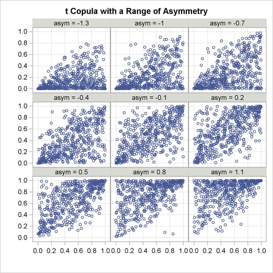
Asymmetrical Copula Example

In this example, an asymmetrical t copula is used to correlate two uniform distributions. The asymmetrical parameter is varied over a range of values to demonstrate its effect. The resulting graphs is produced by using ODS graphics.

data histdata;
   do asym = -1.3 to 1.1 by .3;
      date='01aug2007'd;
      y = .5;
      z = .5;
      output;
   end;
run ;

  /* Add the asymmetric parameter to cov mat */
data asym;
   do asym = -1.3 to 1.1 by .3;
      y = asym;
      z = 0;
      _name_ = "    ";
      _type_ = "asym";
      output;
      y = 1;
      z = .65;
      _name_ = "y";
      _type_ = "cov";
      output;
      y = .65;
      z = 1;
      _name_ = "z";
      _type_ = "cov";
      output;
   end;
run;

proc model out=sim(where=(_REP_ > 0)) data=histdata sdata=asym;
   y = 0;
   errormodel y ~ Uniform(0,1);

   z = 0;
   errormodel z ~ Uniform(0,1);

   solve y z / random=500 seed=12345 copula=(t(5) asym );
   by asym;
run;

To produce a panel plot of this joint distribution, use the following SAS/GRAPH statements.

ods graphics on / height=800 width=800;
proc template;
  define statgraph myplot.panel;
  BeginGraph;
    entrytitle halign=left halign=center
          textattrs=GRAPHTITLETEXT "t Copula with a Range of Asymmetry";

    layout datapanel classvars=(asym) / rows=3 columns=3
          order=rowmajor height=1024 width=1420
          rowaxisopts=(griddisplay=on label=' ')
          columnaxisopts=(griddisplay=on label=' ');
       layout prototype;
          scatterplot x=z y=y ;
       endlayout;
    endlayout;
  EndGraph;
  end;
run;

proc sgrender data=sim template='myplot.panel';
run;

Figure 18.72 t Copula with Asymmetry

Quasi-Random Number Generators

Traditionally high-discrepancy pseudo-random number generators are used to generate innovations in Monte Carlo simulations. Loosely translated, a high-discrepancy pseudo-random number generator is one in which there is very little correlation between the current number generated and the past numbers generated. This property is ideal if indeed independence of the innovations is required. If, on the other hand, the efficient spanning of a multidimensional space is desired, a low discrepancy, quasi-random number generator can be used. A quasi-random number generator produces numbers that have no random component.

A simple one-dimensional quasi-random sequence is the van der Corput sequence. Given a prime number r ( $\text{[math]}$ ), any integer has a unique representation in terms of base r. A number in the interval [0,1) can be created by inverting the representation base power by base power. For example, consider r=3 and n=1, 1 in base 3 is

$\text{[math]}$

When the powers of 3 are inverted,

$\text{[math]}$

Also, 11 in base 3 is

$\text{[math]}$

When the powers of 3 are inverted,

$\text{[math]}$

The first 10 numbers in this sequence $\text{[math]}$ are provided below

$\text{[math]}$

As the sequence proceeds, it fills in the gaps in a uniform fashion.

Several authors have expanded this idea to many dimensions. Two versions supported by the MODEL procedure are the Sobol sequence (QUASI=SOBOL) and the Faure sequence (QUASI=FAURE). The Sobol sequence is based on binary numbers and is generally computationally faster than the Faure sequence. The Faure sequence uses the dimensionality of the problem to determine the number base to use to generate the sequence. The Faure sequence has better distributional properties than the Sobol sequence for dimensions greater than 8.

As an example of the difference between a pseudo-random number and a quasi-random number, consider simulating a bivariate normal with 100 draws.

Figure 18.73 Kernel Density of a Bivariate Normal produced by 100 Faure-Random Draws

Figure 18.74 Kernel Density of a Bivariate Normal produced by 100 Pseudo-Random Draws

Top of Page