PROC SIMILARITY: Similarity Analysis :: SAS/ETS(R) 9.2 User's Guide

The SIMILARITY Procedure

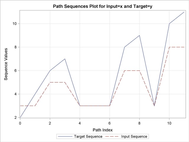
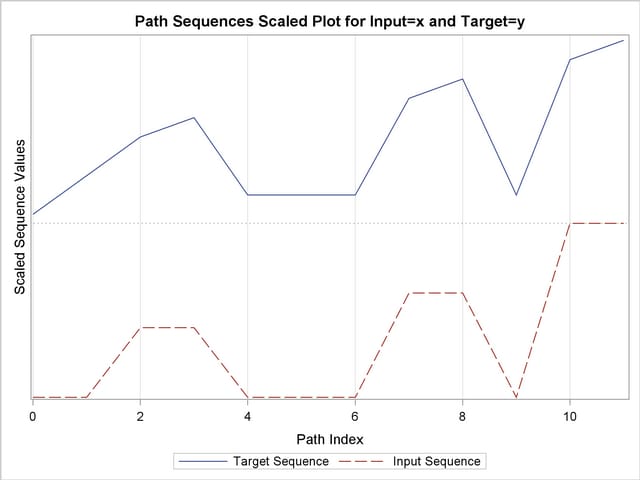
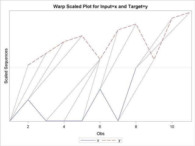
Example 22.2 Similarity Analysis

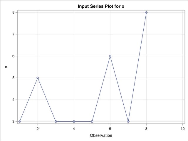
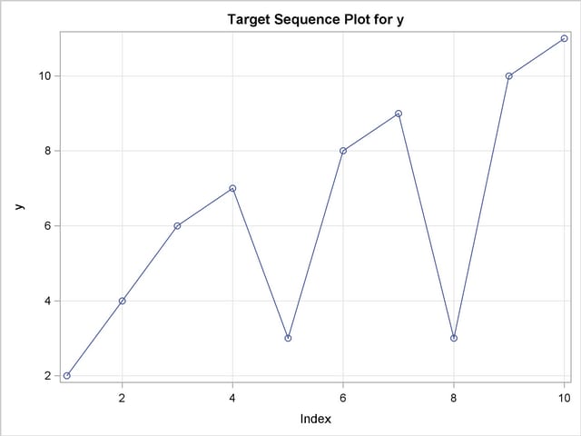
This simple example illustrates how to compare two time sequences using similarity analysis. The following statements create an example data set that contains two time sequences of differing lengths.

   data test;
   input i y x;
   datalines;
   1   2  3
   2   4  5
   3   6  3
   4   7  3
   5   3  3
   6   8  6
   7   9  3
   8   3  8
   9  10  .
   10 11  .
   ;
   run;

The following statements perform similarity analysis on the example data set:

   ods graphics on;
   proc similarity data=test out=_null_
      print=all plot=all;
      input x;
      target y / measure=absdev;
   run;

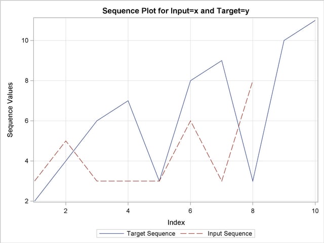
The DATA=TEST option specifies that the input data set WORK.TEST is to be used in the analysis. The OUT=_NULL_ option specifies that no output time series data set is to be created. The PRINT=ALL and PLOTS=ALL options specify that all ODS tables and graphs are to be produced. The INPUT statement specifies that the input variable is X. The TARGET statement specifies that the target variable is Y and that the similarity measure is computed using absolute deviation (MEASURE=ABSDEV).

Output 22.2.1 Description Statistics of the Input Variable, x

The SIMILARITY Procedure

Time Series Descriptive Statistics
Variable	x
Number of Observations	10
Number of Missing Observations	2
Minimum	3
Maximum	8
Mean	4.25
Standard Deviation	1.908627

Output 22.2.2 Plot of Input Variable, x

Output 22.2.3 Target Sequence Plot

Output 22.2.4 Sequence Plot

Output 22.2.5 Path Plot

Output 22.2.6 Path Sequences Plot

Output 22.2.7 Path Sequences Scaled Plot

Output 22.2.8 Path Distance Plot

Output 22.2.9 Path Distance Histogram

Output 22.2.10 Path Relative Distance Plot

Output 22.2.11 Path Relative Distance Histogram

Output 22.2.12 Path Limits

Path Limits
Limit	Specified Absolute	Specified Percentage	Minimum Allowed	Maximum Allowed	Applied
Compression	None	None	2	9	9
Expansion	None	None	0	7	7

Output 22.2.13 Path Statistics

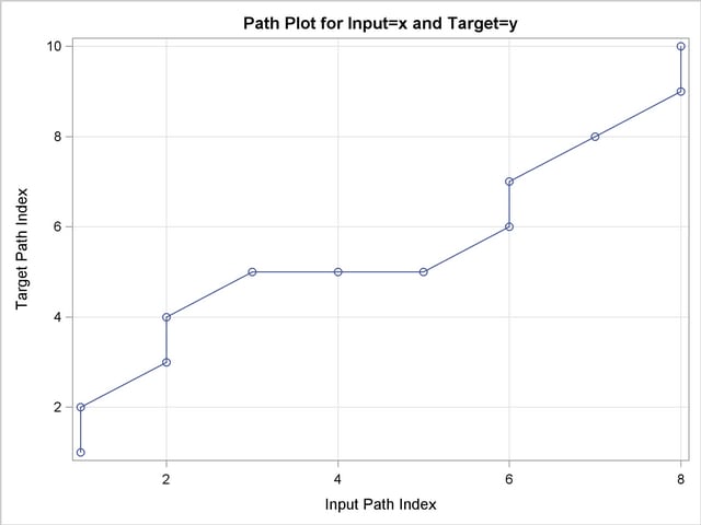
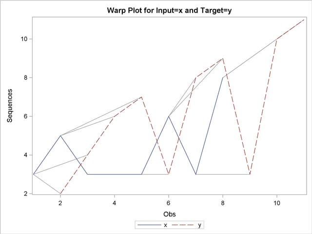
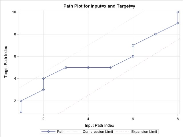
Path Statistics
Path	Number	Path Percent	Input Percent	Target Percent	Maximum	Path Maximum Percent	Input Maximum Percent	Target Maximum Percent
Missing Map	0	0.000%	0.000%	0.000%	0	0.000%	0.000%	0.000%
Direct Maps	6	50.00%	75.00%	60.00%	2	16.67%	25.00%	20.00%
Compression	4	33.33%	50.00%	40.00%	1	8.333%	12.50%	10.00%
Expansion	2	16.67%	25.00%	20.00%	2	16.67%	25.00%	20.00%
Warps	6	50.00%	75.00%	60.00%	2	16.67%	25.00%	20.00%

Output 22.2.14 Cost Plot

Output 22.2.15 Cost Statistics

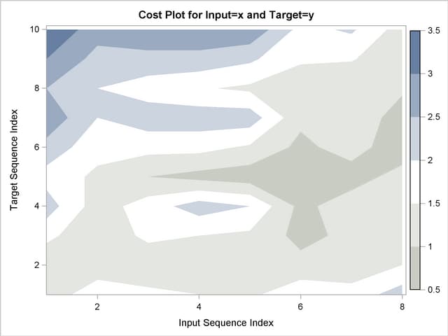
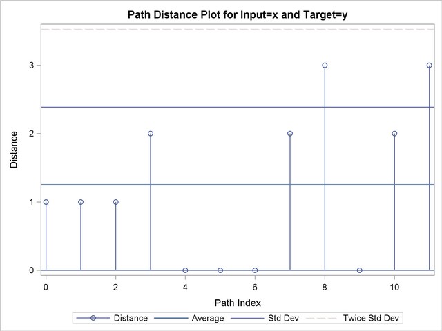
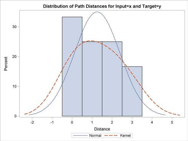
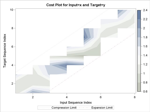
Cost Statistics
Cost	Number	Total	Average	Standard Deviation	Minimum	Maximum	Input Mean	Target Mean	Minimum Path Mean	Maximum Path Mean
Absolute	12	15.00000	1.250000	1.138180	0	3.000000	1.875000	1.500000	1.875000	0.8823529
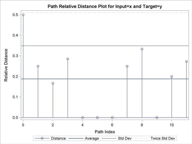
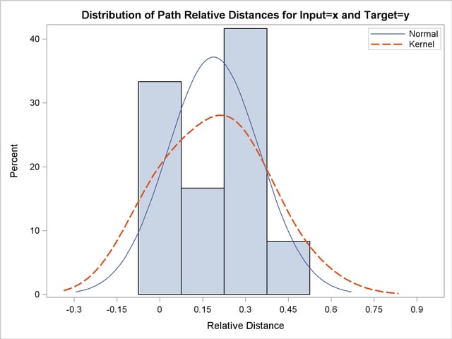
Relative	12	2.25844	0.188203	0.160922	0	0.500000	0.282305	0.225844	0.282305	0.1328495

Relative Costs based on Target Sequence values

Output 22.2.16 Time Warp Plot

Output 22.2.17 Time Warp Scaled Plot

The following statements repeat the above similarity analysis on the example data set with warping limits:

   ods graphics on;
   proc similarity data=test out=_null_
      print=all plot=all;
      input x;
      target y / measure=absdev
      compress=(localabs=2)
      expand=(localabs=2);
   run;

The COMPRESS=(LOCALABS=2) option limits local absolute compression to 2. The EXPAND=(LOCALABS=2) option limits local absolute expansion to 2.

Output 22.2.18 Path Plot with Warping Limits

Output 22.2.19 Warped Path Limits

Path Limits
Limit	Specified Absolute	Specified Percentage	Minimum Allowed	Maximum Allowed	Applied
Compression	2	None	2	9	2
Expansion	2	None	0	7	2

Output 22.2.20 Cost Plot with Warping Limits

The following statements repeat the above similarity analysis on the example data set but store the results in output data sets:

   proc similarity data=test out=series
   outsequence=sequences outpath=path outsum=summary;
   input x;
   target y / measure=absdev
   compress=(localabs=2)
   expand=(localabs=2);
   run;

The OUT=SERIES, OUTSEQUENCE=SEQUENCES, OUTPATH=PATH, and OUTSUM=SUMMARY options specify that the output time series, time sequences, path analysis, and summary data sets be created, respectively.

Note: This procedure is experimental.

Top of Page