The HPCOUNTREG Procedure
-
Overview

- Getting Started
-
Syntax
-
DetailsMissing ValuesPoisson RegressionConway-Maxwell-Poisson RegressionNegative Binomial RegressionZero-Inflated Count Regression OverviewZero-Inflated Poisson RegressionZero-Inflated Conway-Maxwell-Poisson RegressionZero-Inflated Negative Binomial RegressionParameter Naming Conventions for the RESTRICT, TEST, BOUNDS, and INIT StatementsComputational ResourcesCovariance Matrix TypesDisplayed OutputOUTPUT OUT= Data SetOUTEST= Data SetODS Table Names
-
Examples
- References
Zero-Inflated Poisson Regression
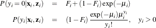
In the zero-inflated Poisson (ZIP) regression model, the data generation process that is referred to earlier as Process 2 is
![\[ g(y_{i}) = \frac{\exp (-\mu _{i})\mu _{i}^{y_{i}}}{y_{i}!} \]](images/etshpug_hpcountreg0158.png)
where  . Thus the ZIP model is defined as
The conditional expectation and conditional variance of  are given by
![\[ E(y_{i}|\mathbf{x}_{i},\mathbf{z}_{i}) = \mu _{i}(1 -F_{i}) \]](images/etshpug_hpcountreg0161.png)
![\[ V(y_{i}|\mathbf{x}_{i},\mathbf{z}_{i}) = E(y_{i}|\mathbf{x}_{i},\mathbf{z}_{i})(1+\mu _{i}F_{i}) \]](images/etshpug_hpcountreg0162.png)
Note that the ZIP model (in addition to the ZINB model) exhibits overdispersion because 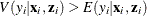 .
.
In general, the log-likelihood function of the ZIP model is
![\[ \mathcal{L} = \sum _{i=1}^{N}\ln \left[ P(y_{i}|\mathbf{x}_{i},\mathbf{z}_{i}) \right] \]](images/etshpug_hpcountreg0164.png)
After a specific link function (either logistic or standard normal) for the probability  is chosen, it is possible to write the exact expressions for the log-likelihood function and the gradient.
ZIP Model with Logistic Link Function
First, consider the ZIP model in which the probability is expressed by a logistic link function, namely
![\[ \varphi _{i}=\frac{\exp (\mathbf{z}_{i}'\bgamma )}{1+\exp (\mathbf{z}_{i}'\bgamma )} \]](images/etshpug_hpcountreg0165.png)
The log-likelihood function is
![\begin{eqnarray*} \mathcal{L} & = & \sum _{\{ i: y_{i}=0\} } \ln \left[\exp (\mathbf{z}_{i}’\bgamma )+\exp (-\exp (\mathbf{x}_{i}’\bbeta )) \right] \\ & & + \sum _{\{ i: y_{i}>0\} }\left[y_{i} \mathbf{x}_{i}’\bbeta -\exp (\mathbf{x}_{i}’\bbeta ) - \sum _{k=2}^{y_{i}}\ln (k) \right] \\ & & - \sum _{i=1}^{N}\ln \left[ 1 + \exp (\mathbf{z}_{i}’\bgamma ) \right] \end{eqnarray*}](images/etshpug_hpcountreg0166.png)
ZIP Model with Standard Normal Link Function
Next, consider the ZIP model in which the probability is expressed by a standard normal link function:  . The log-likelihood function is
![\begin{eqnarray*} \mathcal{L} & = & \sum _{\{ i: y_{i}=0\} } \ln \left\{ \Phi (\mathbf{z}_{i}’\bgamma ) + \left[ 1- \Phi (\mathbf{z}_{i}’\bgamma )\right] \exp (-\exp (\mathbf{x}_{i}’\bbeta )) \right\} \\ & + & \sum _{\{ i: y_{i}>0\} } \left\{ \ln \left[ \left( 1-\Phi (\mathbf{z}_{i}’\bgamma )\right) \right] - \exp (\mathbf{x}_{i}’\bbeta ) + y_{i} \mathbf{x}_{i}’\bbeta - \sum _{k=2}^{y_{i}} \ln (k) \right\} \end{eqnarray*}](images/etshpug_hpcountreg0168.png)
For more information about the zero-inflated Poisson regression model, see the section Zero-Inflated Poisson Regression in SAS/ETS 14.1 User's Guide.