Equivalence Tests

Sample Size and Power Calculations

Equivalence Tests

In a test of equivalence, a treatment mean and a reference mean are compared to each other. Equivalence is taken to be the alternative hypothesis, and the null hypothesis is nonequivalence. The power of a test is the probability of rejecting the null hypothesis when the alternative is true, so in this case, the power is the probability of failing to reject equivalence when the treatments are in fact equivalent, that is, the treatment difference or ratio is within the prespecified boundaries.

The computational details for the power of an equivalence test (refer to Phillips 1990 for the additive model; Diletti, Hauschke, and Steinijans 1991 for the multiplicative) are as follows:

${Power} ={Prob}(t_1 \geq t_{(1-\alpha,\nu)} { and } t_2 \leq -t_{(1-\alpha,\nu)} | {bioequivalence})$

Owen (1965) showed that (t₁, t₂) has a bivariate noncentral t distribution that can be calculated as the difference of two definite integrals (Owen's Q function):

${Power} = Q_{\nu}(-t_{(1-\alpha, \nu)}, \delta_{2}; 0, {\rm R}) - Q_{\nu}(t_{(1-\alpha, \nu)}, \delta_{1}; 0, {\rm R})$

where $t_{(1-\alpha, \nu)}$ is the $(1 - \alpha)$ quantile of a t distribution with $\nu$ df.

$\nu = \{ n - 1 & {for the one-sample and paired tests} \ 2(n - 1) & {for the two-sample test} .$

and

$. \delta_1 = \frac{\theta-b_{l}}{V \cdot \kappa} \ \delta_2 = \frac{\theta-b_{u}}{V \cdot \kappa} \ \theta = {null difference} \} {for the additive model}$

$. \delta_1 = \frac{\log(\theta) -\log(b_l)}{\kappa\sqrt{\log(1+V^2)}} \ \delta... ...\sqrt{\log(1+V^2)}} \ \theta = {null ratio} \} {for the multiplicative model}$

$V & {is the coefficient of variation} \ b_l & {is the lower equivalence bound} \ b_u & {is the upper equivalence bound}$

$\kappa = \{ \sqrt{1/n} & {for the one-sample and paired tests} \ \sqrt{2/n} & {for the two-sample test} \ .$

$R =\frac{\sqrt{\nu}(\delta_1 - \delta_2)}{2 \cdot t_{(1-\alpha,\nu)}}$

For equivalence tests, alpha is usually set to 0.05, and power ranges from 0.70 to 0.90 (often set to 0.80).

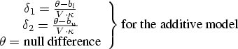
For the additive model of equivalence, the values you must enter for the null difference, the coefficient of variation (c.v.), and the lower and upper bioequivalence limits must be expressed as percentages of the reference mean. More information on specifications follow:

Calculate the null difference as $\frac{|\mu_T - \mu_R|}{\mu_R}$ , where $\mu_T$ is the hypothesized treatment mean and $\mu_R$ is the hypothesized reference mean. The null difference is often in the range of 0 to 0.20.

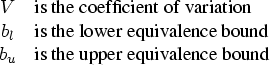
For the coefficient of variation value, $\sigma$ can be estimated by $\hat{\sigma}$ , where $\hat{\sigma}^2$ is the residual variance of the observations (MSE). Enter the c.v. as a percentage of the reference mean, so for the c.v., enter $\frac{\hat{\sigma}}{\mu_R}$ , or $\frac{\sqrt{MSE}}{\mu_R}$ . This value is often in the range of 0.05 to 0.30.

Enter the bioequivalence lower and upper limits as percentages of the reference mean as well. That is, for the bounds, enter $\frac{lower bound}{\mu_R}$ and $\frac{upper bound}{\mu_R}$ . These values are often -0.2 and 0.2, respectively.

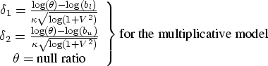
For the multiplicative model of equivalence, calculate the null ratio as $\frac{\mu_T}{\mu_R}$ , where $\mu_T$ is the hypothesized treatment mean and $\mu_R$ is the hypothesized reference mean. This value is often in the range of 0.80 to 1.20. More information on specifications follow:

The coefficient of variation (c.v.) is defined as $\sqrt{e^{(\sigma^2)} -1}$ . You can estimate $\sigma$ by $\hat{\sigma}$ , where $\hat{\sigma}^2$ is the residual variance of the logarithmically transformed observations. That is, $\sigma$ can be estimated by $\sqrt{MSE}$ from the ANOVA of the transformed observations. The c.v. value is often in the range of 0.05 to 0.30.

The bioequivalence lower and upper limits are often set to 0.80 and 1.25, respectively.

Top of Page