Regression

Multiple Linear Regression

You perform a multiple linear regression analysis when you have more than one explanatory variable for consideration in your model. You can write the multiple linear regression equation for a model with p explanatory variables as

Y = b₀ + b₁X₁ + b₂X₂ + ... + b_p X_p

where Y is the response, or dependent, variable, the Xs represent the p explanatory variables, and the bs are the regression coefficients.

For example, suppose that you would like to model a person's aerobic fitness as measured by the ability to consume oxygen. The data set analyzed in this example is named Fitness, and it contains measurements made on three groups of men involved in a physical fitness course at North Carolina State University. See "Computing Correlations" in Chapter 7, "Descriptive Statistics," for a complete description of the variables in the Fitness data set.

The goal of the study is to predict fitness as measured by oxygen consumption. Thus, the dependent variable for the analysis is the variable oxygen. You can choose any of the other quantitative variables (age, weight, runtime, rstpulse, runpulse, and maxpulse) as your explanatory variables.

Suppose that previous studies indicate that oxygen consumption is dependent upon the subject's age, the time it takes to run 1.5 miles, and the heart rate while running. Thus, in order to predict oxygen consumption, you estimate the parameters in the following multiple linear regression equation:

oxygen = b₀ + b₁age+ b₂runtime+ b₃runpulse

This task includes performing a linear regression analysis to predict the variable oxygen from the explanatory variables age, runtime, and runpulse. Additionally, the task requests confidence intervals for the estimates, a collinearity analysis, and a scatter plot of the residuals.

Open the Fitness Data Set

The data are provided in the Analyst Sample Library. To access this data set, follow these steps:

Select Tools Sample Data ...
Select Fitness.
Click OK to create the sample data set in your Sasuser directory.
Select File Open By SAS Name ...
Select Sasuser from the list of Libraries.
Select Fitness from the list of members.
Click OK to bring the Fitness data set into the data table.

Request the Linear Regression Analysis

To specify the analysis, follow these steps:

Select Statistics Regression Linear ...
Select the variable oxygen from the candidate list as the dependent variable.
Select the variables age, runtime, and runpulse as the explanatory variables.

Figure 11.6 displays the resulting Linear Regression task.

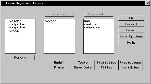Figure 11.6: Linear Regression Dialog

The default analysis fits the linear regression model.

Request Additional Statistics

You can request several additional statistics for your analysis in the Statistics dialog.

To request that confidence limits be computed, follow these steps:

Click on the Statistics button.
In the Statistics tab, select Confidence limits for estimates.

Figure 11.7 displays the Statistics tab in the Statistics dialog.

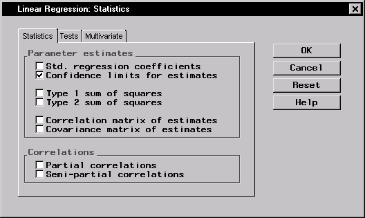Figure 11.7: Linear Regression: Statistics Dialog,Statistics Tab

To request a collinearity analysis, follow these steps:

Click on the Tests tab in the Statistics dialog.
Select Collinearity analysis.
Click OK.

The dialog in Figure 11.8 requests a collinearity analysis in order to assess dependencies among the explanatory variables.

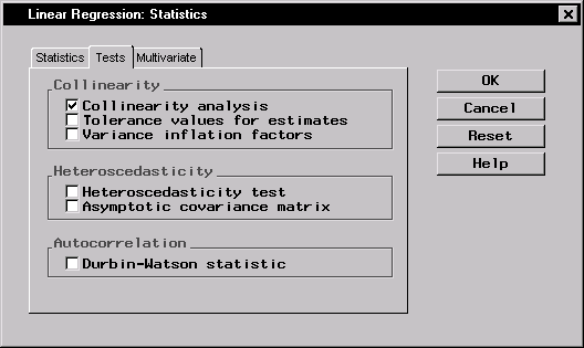Figure 11.8: Linear Regression: Statistics Dialog,Tests Tab

Request a Scatter Plot of the Residuals

To request a plot of the studentized residuals versus the predicted values, follow these steps:

In the Linear Regression main dialog, click on the Plots button.
Click on the Residual tab.
Select Plot residuals vs variables.
In the box labeled Residuals, check the selection Studentized.
In the box labeled Variables, check the selection Predicted Y.
Click OK.

Figure 11.9 displays the Residual tab.

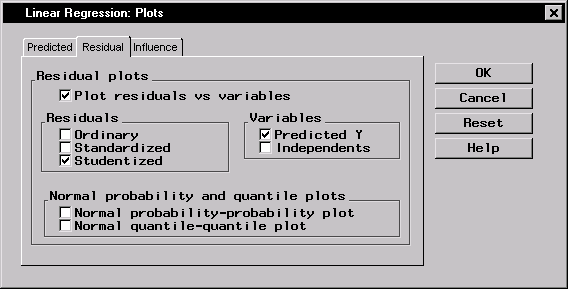Figure 11.9: Linear Regression: Plots Dialog,Residual Tab

An ordinary residual is the difference between the observed response and the predicted value for that response. The standardized residual is the ratio of the residual to its standard error; that is, it is the ordinary residual divided by its standard error. The studentized residual is the standardized residual calculated with the current observation deleted from the analysis.

Click OK in the Linear Regression dialog to perform the analysis.

Review the Results

Figure 11.10 displays the analysis of variance table and the parameter estimates.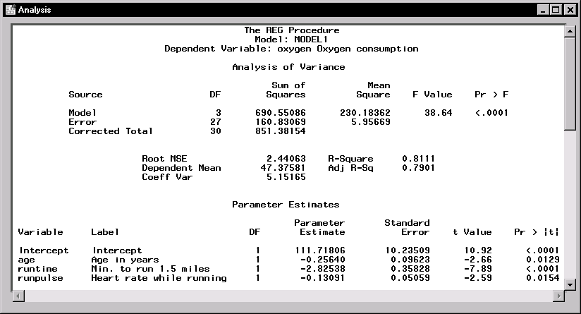

Figure 11.10: Linear Regression: ANOVA Table and Parameter Estimates

In the analysis of variance table displayed in Figure 11.10, the F value of 38.64 (with an associated p-value that is less than 0.0001) indicates a significant relationship between the dependent variable, oxygen, and at least one of the explanatory variables. The R-square value indicates that the model accounts for 81% of the variation in oxygen consumption.

The "Parameter Estimates" table lists the degrees of freedom, the parameter estimates, and the standard error of the estimates. The final two columns of the table provide the calculated t values and associated probabilities (p-values) of obtaining a larger absolute t value. Each p-value is less than 0.05; thus, all parameter estimates are significant at the 5% level. The fitted equation for this model is as follows:

oxygen = 111.718-0.256×age-2.825×runtime-0.131×runpulse

Figure 11.11 displays the confidence limits for the parameter estimates and the table of collinearity diagnostics.

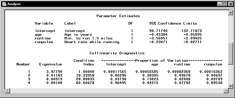Figure 11.11: Linear Regression: Confidence Limits and Collinearity Analysis

The collinearity diagnostics table displays the eigenvalues, the condition index, and the corresponding proportion of variation accounted for in each estimate. Generally, when the condition index is around 10, there are weak dependencies among the regression estimates. When the index is larger than 100, the estimates may have a large amount of numerical error. The diagnostics displayed in Figure 11.11, though indicating unfavorable dependencies among the estimates, are not so excessive as to dismiss the model.

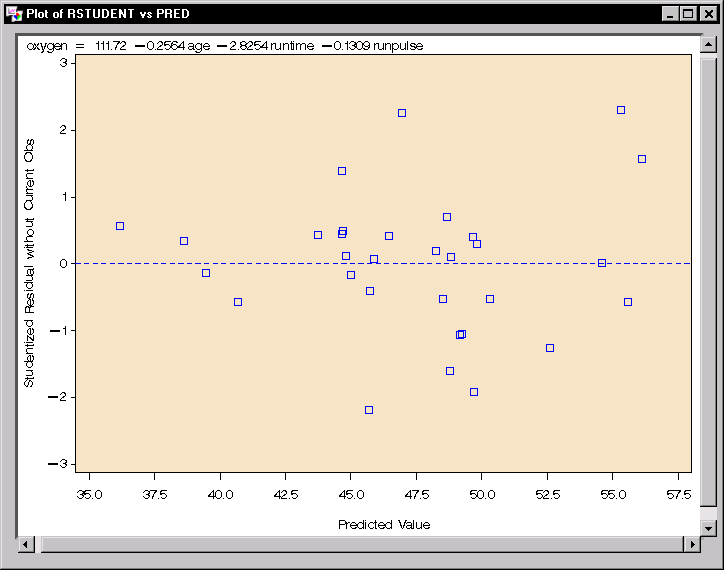Figure 11.12: Linear Regression: Plot of Studentized Residuals versus Predicted Values

The plot of the studentized residuals versus the predicted values is displayed in Figure 11.12. When a model provides a good fit and does not violate any model assumptions, this type of residual plot exhibits no marked pattern or trend. Figure 11.12 exhibits no such trend, indicating an adequate fit.

Top of Page