PDF of Example | SAS/STAT Focus Area Examples

---

Overview

The MCMC procedure in SAS/STAT 14.1 was enhanced with the ability to access lead and lagged values for random variables that are indexed. Two types of random variables in PROC MCMC are indexed: the response (MODEL statement) is indexed by observations, and the random effect (RANDOM statement) is indexed by the SUBJECT= option variable. This new capability extends the range of models that you can fit by using PROC MCMC. For example, you can now fit certain dynamic linear models that were previously inaccessible. In other cases, model specification in PROC MCMC is greatly simplified. For example, to fit autoregressive time series models before this enhancement, you were required to preprocess the data and manually generate variables that contain the lagged values of the response variable. Also, there was no built-in means to account for the initial states of the lagged variables. With the new enhancement, autoregressive time series models no longer require you to preprocess the data, and you can easily specify starting values or prior distributions for the unobserved initial states. What follows are two examples that demonstrate the use of this enhancement to PROC MCMC. The first example fits a fourth-order autoregressive model (AR(4)). The data in the example are simulated in order to avoid the issue of model identification. The second example fits a dynamic linear model with time-varying coefficients to UK coal consumption data, inspired by examples from Congdon (2003) and Harvey (1989). The first example demonstrates the use of lagged values in the MODEL statement, and the second example demonstrates the use of lagged values in the RANDOM statement. Both examples also demonstrate how to produce forecasts by using the PREDDIST statement.

Accessing Lag and Lead Variables In PROC MCMC

Two types of random variables in PROC MCMC are indexed: the response (MODEL statement) is indexed by observations, and the random effect (RANDOM statement) is indexed by the SUBJECT= option variable. As the procedure steps through the input data set, the response or the random-effects symbols are filled with values of the current observation or the random-effects parameters in the current subject. Often you might want to access lag or lead variables across an index. For example, the likelihood function for can depend on in an autoregressive model, or the prior distribution for can depend on , where , in a dynamic linear model. In these situations, you can use the following rules to construct symbols to access values from other observations or subjects:

• rv.Li: the ith lag of the variable rv. This looks back to the past.

• rv.Ni: the ith lead of the variable rv. This looks forward to the future.

The construction is allowed for random variables that are associated with an index, either a response variable or a random-effects variable. You concatenate the variable name, a dot, either the letter L (for “lag”) or the letter N (for “next”), and a lag or a lead number. PROC MCMC resolves these variables according to the indices that are associated with the random variable, with respect to the current observation.

For example, the following RANDOM statement specifies a first-order Markov dependence in the random effect mu that is indexed by the subject variable time:

random mu ~ normal(mu.l1,sd=1) subject=time;

This corresponds to the prior

At each observation, PROC MCMC fills in the symbol mu with the random-effects parameter that belongs to the current cluster t. To fill in the symbol mu.l1, the procedure looks back and finds a lag-1 random-effects parameter, , from the last cluster t–1. As the procedure moves forward in the input data set, these two symbols are constantly updated, as appropriate.

When the index is out of range, such as t–1 when t is 1, PROC MCMC fills in the missing state from the ICOND= option in either the MODEL or RANDOM statement. The following example illustrates how PROC MCMC fills in the values of these lag and lead variables as it steps through the data set.

Assume that the random effect mu has five levels, indexed by . The model contains two lag variables and one lead variable (mu.l1, mu.l2, and mu.n2):

mn = (mu.l1 + mu.l2 + mu.n2) / 3
random mu ~ normal(mn, sd=1) subject=time icond=(alpha beta gamma kappa);

In this setup, instead of a list of five random-effects parameters that the variable mu can be assigned values to, you now have a list of nine variables for the variables mu, mu.l1, mu.l2, and mu.n2. The list lines up in the following order:

PROC MCMC finds relevant symbol values according to this list, as the procedure steps through different subject cluster. The process is illustrated in Table 1.

Table 1: Processing Lag and Lead Variables

sub	mu	mu.l2	mu.l1	mu.n2
a		alpha	beta
b		beta
c
d				gamma
e				kappa

For observations in cluster a, PROC MCMC sets the random-effects variable mu to , looks back two lags and fills in mu.l2 with alpha, looks back one lag and fills in mu.l1 with beta, and looks forward two leads and fills in mu.n2 with . As the procedure moves to observations in cluster b, mu becomes , mu.l2 becomes beta, mu.l1 becomes , and mu.n2 becomes . For observations in the last cluster, cluster e, mu becomes , mu.l2 becomes , mu.l1 becomes , and mu.n2 is filled with kappa.

Autoregressive Model of Order p (AR(p))

The observational equation for an AR(p) model is

where is a constant, are the unknown autoregressive parameters, and . The response variable is assumed to be observed at equally spaced intervals that are indexed by .

If you condition on the unobserved initial states, , then the likelihood for is

Including prior distributions for in the model specification leads to what is known as a full likelihood model (Congdon 2003).

To perform a Bayesian analysis, you assign prior distributions to the unknown quantities . In the following example, the following prior distributions are assigned to these quantities:

Example 1: Simulated AR(4) Model

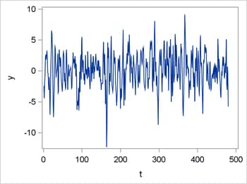
The following example fits an AR(4) model to a simulated time series with , and a sample size of 500. The statements that generate the data are not shown but are included in the sample SAS program file that accompanies this example. A copy of the response variable Y is generated and named X, and then the last 20 observations of Y are set to missing. PROC MCMC automatically imputes values for the missing observations, thus producing an out-of-sample forecast for the response variable. Keeping a copy of the original data stored in X provides the means to assess the accuracy of the out-of-sample forecast.

The following statements generate a plot of the simulated time series Y by using the SGPLOT procedure:

ods graphics on;
proc sgplot data=ar4;
  series x=t y=y;
run;

Figure 1 shows the plot of the time series variable Y.

Figure 1: Simulated AR(4) Time Series

The following statements specify the AR(4) model by using PROC MCMC:

proc mcmc data=ar4 nmc=100000 seed=100 nthreads=8 propcov=quanew;
  parms phi_1 phi_2 phi_3 phi_4;
  parms sigma2 1;
  parms Y_0 Y_1 Y_2 Y_3;
  prior phi_:~normal(0,var=1000);
  prior sigma2 ~ igamma(shape = 3/10, scale = 10/3);
  prior Y_: ~ n(0, var=1000 );
  mu=phi_1*y.l1 + phi_2*y.l2 + phi_3*y.l3 + phi_4*y.l4;
  model y~normal(mu, var=sigma2)
        icond=(Y_3 Y_2 Y_1 Y_0);
  preddist outpred=AR4outpred statistics=brief;
  ods output PredSumInt=AR4PredSumInt;
run;

In the PROC MCMC statement, the NMC= option specifies the number of MCMC iterations, excluding the burn-in iterations; the NTHREADS= option specifies the number of threads to use; and the PROPCOV= option specifies the method to use in constructing the initial covariance matrix for the Metropolis-Hastings algorithm. The QUANEW method finds numerically approximated covariance matrices at the optimum of the posterior density function with respect to all continuous parameters.

The first PARMS statement declares the parameters , , , and and places them in a single parameter block. The second PARMS statement declares the parameter and places it in a separate parameter block. The third PARMS statement specifies that the unobserved initial conditions , , , and be treated as model parameters and places them in a separate parameter block.

The first PRIOR statement specifies normal prior distributions with a mean equal to 0 and a variance equal to 1,000 for the parameters , , , and . The second PRIOR statement specifies an inverse gamma prior distribution with shape equal to 3/10 and a scale equal to 10/3 for the parameter . The third PRIOR statement specifies normal prior distributions with a mean equal to 0 and a variance equal to 1,000 for the initial condition parameters , , , and .

The statement that follows is included strictly for convenience. It specifies , which is the mean of the response variable’s distribution. The quantities y.l1, y.l2, y.l3, and y.l4 represent the first, second, third, and fourth lag of the response variable, respectively.

The MODEL statement specifies that the response variable has a normal distribution with mean and variance . The ICOND= option specifies the initial states of the lag variables for the response variable when the observation indices are out of the range.

In the PREDDIST statement, the OUTPRED= option creates a data set, AR4outpred. that contains random samples from the posterior predictive distribution of the response variable. The STATISTICS=BRIEF option species that posterior means, standard deviations, and the equal-tail intervals be computed. By default, the number of simulated predicted values is the same as the number of simulations that are specified in the NMC= option in the PROC MCMC statement. However, you can specify a different number of simulations by specifying the NSIM= option in the PREDDIST statement. Because the last 20 observations of the response variable are set to missing, PROC MCMC treats those observations as random variables and imputes their values in the predictive distribution. The result is an out-of-sample forecast for the response variable.

The ODS OUTPUT statement specifies that the information from the prediction summaries and intervals table be saved in the data set AR4PredSumInt.

Output 1 displays the posterior summaries and intervals table for the model. The 95% HPD intervals for the parameters , , , , and all contain the true population values, and the means of their respective posterior distributions provide fairly accurate point estimates.

Output 1: Posterior Summaries and Intervals

The MCMC Procedure

Posterior Summaries and Intervals
Parameter	N	Mean	Standard Deviation	95% HPD Interval
phi_1	100000	0.7947	0.0522	0.6945	0.8980
phi_2	100000	-0.5210	0.0630	-0.6467	-0.3987
phi_3	100000	0.4331	0.0628	0.3100	0.5560
phi_4	100000	-0.3674	0.0514	-0.4663	-0.2662
sigma2	100000	4.5998	0.4842	3.7601	5.5631
Y_0	100000	0.9900	5.7539	-9.6331	12.9945
Y_1	100000	0.2228	8.7826	-17.2451	17.5142
Y_2	100000	4.8682	8.9749	-13.4494	22.2866
Y_3	100000	13.6260	9.6851	-5.5431	32.6751

Output 2 shows the effective sample sizes table. The autocorrelation times are high for all the parameters, and the effective sample sizes are small relative to the number of Monte Carlo samples. This evidence indicates slow mixing. However, the trace plots (not shown) provide no evidence that the Markov chain failed to converge.

Output 2: Effective Sample Sizes

The MCMC Procedure

Effective Sample Sizes
Parameter	ESS	Autocorrelation Time	Efficiency
phi_1	6136.4	16.2963	0.0614
phi_2	7259.9	13.7743	0.0726
phi_3	5961.9	16.7731	0.0596
phi_4	4849.7	20.6198	0.0485
sigma2	12298.8	8.1309	0.1230
Y_0	7265.8	13.7631	0.0727
Y_1	6758.8	14.7956	0.0676
Y_2	6487.0	15.4154	0.0649
Y_3	6319.7	15.8236	0.0632

The following statements merge the original data set Ar4 with the ODS OUTPUT data set AR4PredSumInt and then use PROC SGPLOT to plot the original in-sample series, the in-sample prediction, the out-of-sample forecast, and a 95% HPD interval around the forecast. Only the last 100 observations are used in the plot to make it easier to visually assess the model fit and the accuracy of the forecast.

data ar4forecast;
  merge ar4 AR4PredSumInt;
run;

proc sgplot data=ar4forecast(where=(t>400));
  series x=t y=y / lineattrs=(color=red);
  series x=t y=x / lineattrs=(color=red pattern=dot);
  series x=t y=mean / lineattrs=(color=blue pattern=dash);
  band x=t upper=hpdupper lower=hpdlower / transparency=.5;
run;

Figure 2 shows the resulting plots. The solid red line represents the original in-sample response variable; the dotted red line represents the out-of-sample values of the response variable; the dashed blue line represents the mean of the predictive distribution; and the light blue shaded area represents the 95% HPD interval. As is typical of linear autoregressive models, the forecasts tend to lag at turning points, and the out-of-sample forecast accuracy diminishes as you forecast further into the future. Because the data are simulated with known population parameter values, model identification is not an issue. Thus, models such as this one provide a useful qualitative benchmark with which to compare the performance of models of "real world" data, where model identification is uncertain.

Figure 2: Forecast of Simulated AR(4) Time Series

Dynamic Linear Model with Time-Varying Coefficients

Dynamic linear models with time-varying coefficients enable you to model stochastic shifts in regression parameters. This is accomplished by using random-effects models that specify time dependence between successive parameter values in the form of smoothness priors. For example, the following describes a smoothing model that appears in Congdon (2003, p. 207) for a time series with seasonal effects and a secular trend:

The first equation states that the response variable is normally distributed and the mean of the distribution is indexed by time, implying that the response variable is nonstationary. The second equation states that the mean of the response variable consists of a trend plus seasonal effects. The third equation states that the trend follows a random walk plus drift. The fourth equation states that the drift term follows a first-order autoregressive process. The fifth equation states that the seasonal effect is a normally distributed random shock whose mean equals the negated sum of the three previous shocks.

To perform a Bayesian analysis, you assign prior distributions to the unknown quantities and , which are the initial states of and , respectively; , , and , which are the initial states of ; , , , and , which are the unknown variances of , , , and , respectively; , which is the first-order autoregressive parameter that modifies in the mean of ; and , which is the variance of . The following prior distributions are assigned to these quantities in the example that follows:

Example 2: UK Coal Consumption

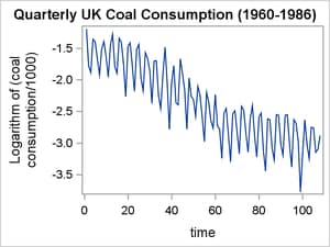
This example fits a time-varying coefficients model to observed quarterly coal consumption in the United Kingdom for the years 1960–1986. It is based on an example that is published in Congdon (2003, p. 207), which in turn is based on a model and data that are published in Harvey (1989). The following statements create the data set UKcoal, which contains the variables Coal, C, Year, Quarter, and T. The variable Coal measures quarterly coal consumption. C is a variance-stabilizing transformation of Coal; specifically, it is the natural logarithm of Coal divided by 1,000. The variables Year and Quarter represent the years and quarters of the observations. The variable T indexes the observations.

The following statements plot the original coal consumption series and the transformed series:

proc sgplot data=UKcoal;
  title "Quarterly UK Coal Consumption (1960-1986)";
  series y=coal x=t;
  yaxis label="Coal consumption";
  xaxis label="time";
run;
title;

proc sgplot data=UKcoal;
  title "Quarterly UK Coal Consumption (1960-1986)";
  series y=c x=t;
  yaxis label="Logarithm of (coal consumption/1000)";
  xaxis label="time";
run;
title;

Figure 3 displays the original coal consumption time series on the left and the transformed coal consumption time series on the right. It appears that the logarithmic transformation has successfully made the variance of the series more homogeneous.

Figure 3: Quarterly UK Coal Consumption (1960–1986)

Raw Data	Transformed Data

The following DATA step creates the variable Z, which is just a copy of C. After Z is created, Coal is set to missing for the years 1985–1986 to enable you to assess the accuracy of the model’s out-of-sample forecast.

data UKcoal;
  set UKcoal;
  z=c;
  if year>1984 then c=.;
run;

The following statements use PROC MCMC to fit the time-varying coefficients model:

proc mcmc data=UKcoal nmc=100000 seed=123456 outpost=posterior propcov=quanew;
  parms alpha0;
  parms mu0;
  parms s0 s1 s2;
  parms theta1;
  parms theta2;
  parms theta3;
  parms theta4;
  parms theta_phi;
  parms phi;
  prior phi~normal(0,var=exp(theta_phi));
  prior alpha0~normal(0,var=theta2);
  prior mu0~normal(0,var=100);
  prior s:~normal(0,var=theta3);
  prior theta:~igamma(shape = 3/10, scale = 10/3);
  random alpha~normal(phi*alpha.l1,var=exp(theta2)) subject=t icond=(alpha0);
  random s~normal(-s.l1-s.l2-s.l3,var=exp(theta3)) subject=quarter icond=(s2 s1 s0);
  random mu~normal(mu.l1 + alpha.l1,var=exp(theta1)) subject=t icond=(mu0);
  x=mu + s;
  model c~normal(x,var=exp(theta4));
  preddist outpred=TVCoutpred statistics=brief;
  ods output PredSumInt=TVCPredSumInt;
run;

In the PROC MCMC statement, the NMC= option specifies the number of MCMC iterations, excluding the burn-in iterations; the PROPCOV= option specifies the method to use in constructing the initial covariance matrix for the Metropolis-Hastings algorithm. The QUANEW method finds numerically approximated covariance matrices at the optimum of the posterior density function with respect to all continuous parameters.

The nine PARMS statements declare the model parameters. The three seasonal parameters , , and are placed in the same block; experimentation with this model and these data showed that putting all the other parameters in separate blocks improved the mixing.

The first PRIOR statement specifies a normal prior distribution for the parameter , with mean equal to 0 and variance equal to . Experimentation with this model and these data showed that sampling the parameter on the logarithmic scale significantly improved mixing. The second PRIOR statement specifies a normal prior distribution for the parameter , with mean equal to 0 and variance equal to the parameter ; represents the initial state of the first-order autoregressive drift component. The third PRIOR statement specifies a normal prior distribution for the parameter , with mean equal to 0 and variance equal to 1,000; represents the initial state for . The fourth PRIOR statement specifies normal prior distributions for , , and , with means equal to 0 and variances equal to the parameter ; , , and represent the initial states for the seasonal random effect . The fifth PRIOR statement specifies inverse gamma distributions for the variance parameters , , , , and . All these distributions have shape and scale parameters specified to be 3/10 and 10/3, respectively.

The first RANDOM statement specifies that the random effect has a normal prior distribution, with a mean equal to the product of and the first lag of and a variance equal to . Experimentation with this model and these data showed that sampling on the logarithmic scale significantly improved mixing. The SUBJECT= option specifies that the random effect is indexed by the variable T. The ICOND= option specifies that the initial state of is represented by the parameter .

The second RANDOM statement specifies that the seasonal random effect has a normal prior distribution, with a mean equal to and a variance equal to . Experimentation with this model and these data showed that sampling on the logarithmic scale significantly improved mixing. The SUBJECT= option specifies that the random effect is indexed by the variable Quarter. The ICOND= option specifies that the initial states of are represented by the parameters , , and .

The third RANDOM statement specifies that the trend random effect has a normal prior distribution, with a mean equal to and a variance equal to . Experimentation with this model and these data showed that sampling on the logarithmic scale significantly improved mixing. The SUBJECT= option specifies that the random effect is indexed by the variable T. The ICOND= option specifies that the initial state of is represented by the parameter .

The next statement is included primarily for convenience. It specifies that , the mean of the response variable’s distribution, is equal to .

The MODEL statement specifies that the response variable has a normal distribution, with a mean equal to and a variance equal to . Experimentation with this model and these data showed that sampling on the logarithmic scale significantly improved mixing.

The PREDDIST statement specifies that the random samples from the predictive distribution be saved in the data set TVCoutpred. The STATISTICS=BRIEF option specifies that the posterior means, standard deviations, and equal-tail intervals be computed. The NSIM= option is omitted, so the number of iterations defaults to the number that is specified in the NMC= option in the PROC MCMC statement.

The ODS OUTPUT statement specifies that the information from the prediction summaries and intervals table be saved in the data set TVCPredSumInt.

Output 3 shows the posterior summaries and intervals table for the time-varying coefficients model, and Output 4 shows the effective sample sizes. The autocorrelation times are relatively large, indicating slow mixing. This is the reason that the number of MCMC iterations was set to the relatively large value of 100,000.

Output 3: Posterior Summaries and Intervals

The MCMC Procedure

Posterior Summaries and Intervals
Parameter	N	Mean	Standard Deviation	95% HPD Interval
alpha0	100000	-0.00141	0.6895	-1.3397	1.3774
mu0	100000	-1.4996	1.8070	-4.8613	2.2364
s0	100000	-0.0202	1.0511	-2.1555	2.0876
s1	100000	-0.0896	1.0811	-2.2344	2.1274
s2	100000	-0.0536	1.1248	-2.3323	2.1594
theta1	100000	0.4690	0.1156	0.2620	0.7038
theta2	100000	0.4917	0.1223	0.2660	0.7339
theta3	100000	1.5701	0.7386	0.4389	3.0281
theta4	100000	0.4234	0.1012	0.2390	0.6230
theta_phi	100000	2.7582	1.6956	0.5189	6.1682
phi	100000	-0.3280	0.1954	-0.7009	0.0557

Output 4: Effective Sample Size

The MCMC Procedure

Effective Sample Sizes
Parameter	ESS	Autocorrelation Time	Efficiency
alpha0	8829.0	11.3263	0.0883
mu0	2635.0	37.9511	0.0263
s0	2256.6	44.3139	0.0226
s1	8318.4	12.0215	0.0832
s2	7972.2	12.5436	0.0797
theta1	10565.8	9.4645	0.1057
theta2	5391.2	18.5489	0.0539
theta3	1696.3	58.9535	0.0170
theta4	9771.8	10.2336	0.0977
theta_phi	10643.7	9.3952	0.1064
phi	2136.4	46.8074	0.0214

he following statements merge the original data set, UKcoal, with the ODS OUTPUT data set TVCPredSumInt and then use PROC SGPLOT to plot the original in-sample series, the in-sample prediction, the out-of-sample forecast, and a 95% HPD interval around the forecast:

data forecast;
  merge UKcoal TVCPredSumInt;
run;

proc sgplot data=forecast;
  series x=t y=c / lineattrs=(color=red);
  series x=t y=z / lineattrs=(color=red pattern=dot);
  series x=t y=mean / lineattrs=(color=blue pattern=dash);
  band x=t upper=hpdupper lower=hpdlower / transparency=.5;
run;

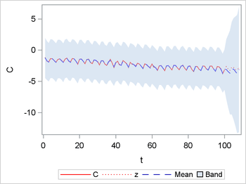
Figure 4 shows the resulting plots. The solid red line represents the original in-sample response variable; the dotted red line represents the out-of-sample values of the response variable; the dashed blue line represents the mean of the predictive distribution; and the light blue shaded area represents the 95% HPD interval. The in-sample model prediction appears to fit the data. The out-of-sample forecast likewise appears to perform well. The 95% HPD interval around the out-of-sample forecast grows very quickly, indicating, not unexpectedly, that the further out of sample you forecast, the greater the uncertainty of the forecast.

Figure 4: Forecast of Quarterly UK Coal Consumption (1960–1986)

References

• Congdon, P. (2003). Applied Bayesian Modeling. New York: John Wiley & Sons.

• Harvey, A. C. (1989). Forecasting, Structural Time Series Models, and the Kalman Filter. Cambridge: Cambridge University Press.

---

These sample files and code examples are provided by SAS Institute Inc. "as is" without warranty of any kind, either express or implied, including but not limited to the implied warranties of merchantability and fitness for a particular purpose. Recipients acknowledge and agree that SAS Institute shall not be liable for any damages whatsoever arising out of their use of this material. In addition, SAS Institute will provide no support for the materials contained herein.

---

%let N = 500;
%let p = 4;
%let sigma=2;
%let constant = 0;
data ar4(keep= t y);
  call streaminit(12345);
  array phi phi1 - phi&p (.8, -.64, .512, -.4096);
  array yLag   yLag1 - yLag&p;
  do j = 1 to dim(yLag);
    yLag[j] = 0;
  end;
  constant=&constant;
  do t = -100 to &N;
    e = rand('normal',0,&sigma);
    y = e;
    do j = 1 to dim(phi);
      y = y + phi[j] * yLag[j];
    end;
    y=y+constant;
    if t > 0 then output;
    do j = dim(yLag) to 2 by -1;
      yLag[j] = yLag[j-1];
    end;
    yLag[1] = y;
  end;
run;

data ar4;
  set ar4;
  x=y;
  if t>480 then y=.;
run;


ods graphics on;
proc sgplot data=ar4;
  series x=t y=y;
run;


proc mcmc data=ar4 nmc=100000 seed=100 nthreads=8 propcov=quanew;
  parms phi_1 phi_2 phi_3 phi_4;
  parms sigma2 1;
  parms Y_0 Y_1 Y_2 Y_3;
  prior phi_:~normal(0,var=1000);
  prior sigma2 ~ igamma(shape = 3/10, scale = 10/3);
  prior Y_: ~ n(0, var=1000 );
  mu=phi_1*y.l1 + phi_2*y.l2 + phi_3*y.l3 + phi_4*y.l4;
  model y~normal(mu, var=sigma2)
        icond=(Y_3 Y_2 Y_1 Y_0);
  preddist outpred=AR4outpred statistics=brief;
  ods output PredSumInt=AR4PredSumInt;
run;


data ar4forecast;
  merge ar4 AR4PredSumInt;
run;


proc sgplot data=ar4forecast(where=(t>400));
  series x=t y=y / lineattrs=(color=red);
  series x=t y=x / lineattrs=(color=red pattern=dot);
  series x=t y=mean / lineattrs=(color=blue pattern=dash);
  band x=t upper=hpdupper lower=hpdlower / transparency=.5;
run;


data UKcoal;
  input coal year quarter @@;
  t=_N_;
  C=log(coal/1000);
  datalines;
303 1960 1 169 1960 2 152 1960 3 257 1960 4
247 1961 1 189 1961 2 146 1961 3 220 1961 4
248 1962 1 195 1962 2 141 1962 3 235 1962 4
278 1963 1 167 1963 2 150 1963 3 261 1963 4
244 1964 1 174 1964 2 104 1964 3 228 1964 4
243 1965 1 170 1965 2 113 1965 3 219 1965 4
237 1966 1 138 1966 2 114 1966 3 208 1966 4
190 1967 1 157 1967 2 93  1967 3 182 1967 4
183 1968 1 106 1968 2 86  1968 3 144 1968 4
226 1969 1 128 1969 2 62  1969 3 130 1969 4
169 1970 1 94  1970 2 91  1970 3 188 1970 4
148 1971 1 114 1971 2 62  1971 3 139 1971 4
104 1972 1 99  1972 2 76  1972 3 122 1972 4
107 1973 1 76  1973 2 51  1973 3 111 1973 4
95  1974 1 71  1974 2 63  1974 3 107 1974 4
65  1975 1 62  1975 2 39  1975 3 80  1975 4
86  1976 1 57  1976 2 37  1976 3 79  1976 4
83  1977 1 59  1977 2 42  1977 3 89  1977 4
84  1978 1 59  1978 2 43  1978 3 73  1978 4
90  1979 1 56  1979 2 40  1979 3 75  1979 4
80  1980 1 45  1980 2 32  1980 3 73  1980 4
72  1981 1 46  1981 2 38  1981 3 78  1981 4
77  1982 1 49  1982 2 41  1982 3 77  1982 4
78  1983 1 49  1983 2 34  1983 3 72  1983 4
68  1984 1 51  1984 2 23  1984 3 42  1984 4
72  1985 1 49  1985 2 39  1985 3 64  1985 4
63  1986 1 43  1986 2 45  1986 3 56  1986 4
;


proc sgplot data=UKcoal;
  title "Quarterly UK Coal Consumption (1960-1986)";
  series y=coal x=t;
  yaxis label="Coal consumption";
  xaxis label="time";
run;
title;


proc sgplot data=UKcoal;
  title "Quarterly UK Coal Consumption (1960-1986)";
  series y=c x=t;
  yaxis label="Logarithm of (coal consumption/1000)";
  xaxis label="time";
run;
title;


data UKcoal;
  set UKcoal;
  z=c;
  if year>1984 then c=.;
run;


proc mcmc data=UKcoal nmc=100000 seed=123456 outpost=posterior propcov=quanew;
  parms alpha0;
  parms mu0;
  parms s0 s1 s2;
  parms theta1;
  parms theta2;
  parms theta3;
  parms theta4;
  parms theta_phi;
  parms phi;
  prior phi~normal(0,var=exp(theta_phi));
  prior alpha0~normal(0,var=theta2);
  prior mu0~normal(0,var=100);
  prior s:~normal(0,var=theta3);
  prior theta:~igamma(shape = 3/10, scale = 10/3);
  random alpha~normal(phi*alpha.l1,var=exp(theta2)) subject=t icond=(alpha0);
  random s~normal(-s.l1-s.l2-s.l3,var=exp(theta3)) subject=quarter icond=(s2 s1 s0);
  random mu~normal(mu.l1 + alpha.l1,var=exp(theta1)) subject=t icond=(mu0);
  x=mu + s;
  model c~normal(x,var=exp(theta4));
  preddist outpred=TVCoutpred statistics=brief;
  ods output PredSumInt=TVCPredSumInt;
run;


data forecast;
  merge UKcoal TVCPredSumInt;
run;

proc sgplot data=forecast;
  series x=t y=c / lineattrs=(color=red);
  series x=t y=z / lineattrs=(color=red pattern=dot);
  series x=t y=mean / lineattrs=(color=blue pattern=dash);
  band x=t upper=hpdupper lower=hpdlower / transparency=.5;
run;

---

These sample files and code examples are provided by SAS Institute Inc. "as is" without warranty of any kind, either express or implied, including but not limited to the implied warranties of merchantability and fitness for a particular purpose. Recipients acknowledge and agree that SAS Institute shall not be liable for any damages whatsoever arising out of their use of this material. In addition, SAS Institute will provide no support for the materials contained herein.

The MCMC procedure in SAS/STAT 14.1 was enhanced with the ability to access lead and lagged values for random variables that are indexed.

Type:	Sample
Topic:	SAS Reference ==> Procedures ==> MCMC Analytics ==> Bayesian Analysis

Date Modified:	2017-01-13 14:43:22
Date Created:	2017-01-13 14:10:35

Operating System and Release Information

Product Family	Product	Host	Product Release		SAS Release
			Starting	Ending	Starting	Ending
SAS System	SAS/STAT	z/OS	14.1		9.4 TS1M3
		z/OS 64-bit	14.1		9.4 TS1M3
		Microsoft® Windows® for x64	14.1		9.4 TS1M3
		Microsoft Windows 8 Enterprise 32-bit	14.1		9.4 TS1M3
		Microsoft Windows 8 Enterprise x64	14.1		9.4 TS1M3
		Microsoft Windows 8 Pro 32-bit	14.1		9.4 TS1M3
		Microsoft Windows 8 Pro x64	14.1		9.4 TS1M3
		Microsoft Windows 8.1 Enterprise 32-bit	14.1		9.4 TS1M3
		Microsoft Windows 8.1 Enterprise x64	14.1		9.4 TS1M3
		Microsoft Windows 8.1 Pro 32-bit	14.1		9.4 TS1M3
		Microsoft Windows 8.1 Pro x64	14.1		9.4 TS1M3
		Microsoft Windows 10	14.1		9.4 TS1M3
		Microsoft Windows Server 2008	14.1		9.4 TS1M3
		Microsoft Windows Server 2008 R2	14.1		9.4 TS1M3
		Microsoft Windows Server 2008 for x64	14.1		9.4 TS1M3
		Microsoft Windows Server 2012 Datacenter	14.1		9.4 TS1M3
		Microsoft Windows Server 2012 R2 Datacenter	14.1		9.4 TS1M3
		Microsoft Windows Server 2012 R2 Std	14.1		9.4 TS1M3
		Microsoft Windows Server 2012 Std	14.1		9.4 TS1M3
		Windows 7 Enterprise 32 bit	14.1		9.4 TS1M3
		Windows 7 Enterprise x64	14.1		9.4 TS1M3
		Windows 7 Home Premium 32 bit	14.1		9.4 TS1M3
		Windows 7 Home Premium x64	14.1		9.4 TS1M3
		Windows 7 Professional 32 bit	14.1		9.4 TS1M3
		Windows 7 Professional x64	14.1		9.4 TS1M3
		Windows 7 Ultimate 32 bit	14.1		9.4 TS1M3
		Windows 7 Ultimate x64	14.1		9.4 TS1M3
		64-bit Enabled AIX	14.1		9.4 TS1M3
		64-bit Enabled Solaris	14.1		9.4 TS1M3
		HP-UX IPF	14.1		9.4 TS1M3
		Linux for x64	14.1		9.4 TS1M3
		Solaris for x64	14.1		9.4 TS1M3