Sample 45570: Bayesian Linear Regression with Standardized Covariates
 |  |  |  |
Analysis
The following data set contains salary and performance information for Major League Baseball players (excluding pitchers) who played at least one game in both the 1986 and 1987 seasons. The salaries are for the 1987 season (Time Inc.; 1987 ) , and the performance measures are from the 1986 season (Reichler; 1987 ) .
data baseball;
   input logSalary no_hits no_runs no_rbi no_bb yr_major cr_hits @@;
   yr_major2 = yr_major*yr_major;
   cr_hits2  = cr_hits*cr_hits;
   label no_hits="Hits in 1986" no_runs="Runs in 1986"
         no_rbi="RBIs in 1986"  no_bb="Walks in 1986"
         yr_major="Years in MLB" cr_hits="Career Hits"
         yr_major2="Years in MLB^2" cr_hits2="Career Hits^2"
         logSalary = "log10(Salary)";
   datalines;
           .  66 30 29 14  1   66
2.6766936096  81 24 38 39 14  835

   ... more lines ...

  2.84509804 127 65 48 37  5  806
 2.942008053 136 76 50 94 12 1511
2.5854607295 126 61 43 52  6  433
 2.982271233 144 85 60 78  8  857
           3 170 77 44 31 11 1457
;
The MEANS procedure produces summary statistics for these data. Summary measures are saved to the SUM_BASEBALL data set for future analysis.
proc means data = baseball mean stddev;
   output out=sum_baseball(drop=_type_ _freq_);
run;
Figure 1 displays the results.
| Variable | Label | Mean | Std Dev | ||||||||||||||||||||||||||||||||||||
|---|---|---|---|---|---|---|---|---|---|---|---|---|---|---|---|---|---|---|---|---|---|---|---|---|---|---|---|---|---|---|---|---|---|---|---|---|---|---|---|
|
|
|
|
Bayesian Linear Regression Model
Suppose you want to fit a Bayesian linear regression model for the logarithm of a player’s salary with density as follows:

|

|

|
|||

|

|

|
( 1 ) |
where
 is the vector of covariates listed as
 for
for
 baseball players. Pete Rose was an extreme outlier in 1986, and his information greatly skews results. He is omitted from this data set and analysis.
The likelihood function for the logarithm of salary and the corresponding covariates is

|
|

|
( 2 ) |
where
 denotes a conditional probability density. The normal density is evaluated at the specified value of
 and the corresponding mean parameter
 defined in Equation
1
. The regression parameters in the likelihood are
defined in Equation
1
. The regression parameters in the likelihood are
 through
 .
.
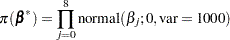
Suppose the following prior distributions are placed on the parameters:

|
|
|
|||

|
|

|
( 3 ) |
where
 indicates a prior distribution and
 is the density function for the inverse-gamma distribution. Priors of this type with large variances are often called
diffuse
priors.
is the density function for the inverse-gamma distribution. Priors of this type with large variances are often called
diffuse
priors.
Using Bayes’ theorem, the likelihood function and prior distributions determine the posterior distribution of the parameters as follows:

|
PROC MCMC obtains samples from the desired posterior distribution. You do not need to specify the exact form of the posterior distribution.
The following SAS statements use the likelihood function and prior distributions to fit the Bayesian linear regression model. The PROC MCMC statement invokes the procedure and specifies the input data set. The NBI= option specifies the number of burn-in iterations. The NMC= option specifies the number of posterior simulation iterations. The SEED= option specifies a seed for the random number generator (the seed guarantees the reproducibility of the random stream). The PROPCOV=QUANEW option uses the estimated inverse Hessian matrix as the initial proposal covariance matrix.
ods graphics on;
proc mcmc data=baseball nbi=50000 nmc=10000 seed=1181 propcov=quanew;
array beta[9] beta0-beta8;
array data[9] 1 no_hits no_runs no_rbi no_bb
yr_major cr_hits yr_major2 cr_hits2;
parms beta: 0;
parms sig2 1;
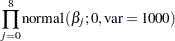
prior beta: ~ normal(0,var = 1000);
prior sig2 ~ igamma(shape = 3/10, scale = 10/3);
call mult(beta, data, mu);
model logsalary ~ n(mu, var = sig2);
run;
ods graphics off;
Each of the two ARRAY statements associates a name with a list of variables and constants. The first ARRAY statement specifies names for the regression coefficients. The second ARRAY statement contains all of the covariates.
The first PARMS statement places all regression parameters in a single block and assigns them an initial value of 0. The second PARMS statement places the variance parameter in a separate block and assigns it an initial value of 1.
The first PRIOR statement assigns the normal prior to each of the regression parameters. The second PRIOR statement assigns the inverse-gamma prior distribution to
 .
.
The CALL statement uses the MULT matrix multiplication function to calculate
. The MODEL statement specifies the likelihood function as given in Equation
2
.
The first step in evaluating the results is to review the convergence diagnostics. With ODS Graphics turned on, PROC MCMC produces graphs.
Figure 2
displays convergence diagnostic graphs for the
regression parameter. The trace plot indicates that the chain does not appear to have reached a stationary distribution and appears to have poor mixing. The diagnostic plots for the rest of the parameters (not shown here) tell a similar story.
Figure 2
Bayesian Diagnostic Plots for


The non-convergence exhibited here results because the parameters are scaled very differently from each other for these data. The random walk Metropolis algorithm is not an optimal sampling algorithm in the case where the parameters have vastly different scales. Standardized covariates (Mayer and Younger; 1976 ) eliminate this problem, and the random walk Metropolis algorithm proceeds smoothly.
Bayesian Linear Regression Model with Standardized Covariates
Suppose you want to fit the same Bayesian linear regression model, but you want to use standardized covariates. You rewrite the mean function in Equation 1 as

|
|

|
where
 is the design matrix constructed from a column of 1s and
 standardized covariates. The regression parameters on the standardized scale are represented by
 . The standardized covariates are computed as follows:

|
|

|
for
 players and
 covariates, and where
 and
and
 are the mean and standard deviation of the
 th covariate, respectively.
The following statements manipulate the SUM_BASEBALL output data set from the earlier use of PROC MEANS. The statements create macro variables for the means and standard deviations to use later in the analysis. The macro variables are independent of SAS data set variables and can be referenced in SAS procedures to facilitate computations. The TRANSPOSE procedure transposes the SUM_BASEBALL data set and a DATA step creates the macro variables by using the SYMPUTX functions. The %PUT statements enable you to verify that the macro variables have been created successfully.
proc transpose data=sum_baseball out=tab;
   id _stat_;
run;

data _null_;
   set tab;
   sub = put((_n_-1), 1.);
   call symputx(compress('m' || sub,'*'), mean);
   call symputx(compress('s' || sub,'*'), std);
run;

%put &m1 &m2 &m3 &m4 &m5 &m6 &m7 &m8;
%put &s1 &s2 &s3 &s4 &s5 &s6 &s7 &s8;
In this example,
and
were calculated in the MEANS procedure and recorded in the macro variables M1–M8 and S1–S8, respectively. The STANDARD procedure computes standardized values of the variables in the original data set.
proc standard data=baseball out=baseball_std mean=0 std=1;
   var no_hits -- cr_hits2;
run;
The new likelihood function for the logarithm of the salary and corresponding standardized covariates is as follows:

|
|

|
For ease of interpretation and inference, you can transform the standardized regression parameters back to the original scale with the following formulas:

|
|

|
|||

|

|

|
|||

|
|

|
|||

|
|

|
Suppose the following diffuse prior distribution is placed on
:
|
The prior distribution for
is given in Equation
3
.
Using Bayes' theorem, the likelihood function and prior distributions determine the posterior distribution of the parameters as follows:

|
The following SAS statements fit the Bayesian linear regression model. The MONITOR= option outputs analysis on selected symbols of interest in the program.
ods graphics on;
proc mcmc data=baseball_std nbi=10000 nmc=20000 seed=1181
   propcov=quanew monitor=(beta0-beta8 sig2);
   array beta[9] beta0-beta8 (0);
   array betastar[9] betastar0-betastar8;
   array data[9] 1 no_hits  no_runs  no_rbi no_bb
      yr_major cr_hits yr_major2 cr_hits2;
   array mn[9] (0 &m1 &m2 &m3 &m4 &m5 &m6 &m7 &m8);
   array std[9] (0 &s1 &s2 &s3 &s4 &s5 &s6 &s7 &s8);

   parms betastar: 0;
   parms sig2 1;

   prior betastar: ~ normal(0,var = 1000);
   prior sig2 ~ igamma(shape = 3/10, scale = 10/3);

   call mult(betastar, data, mu);
   model logsalary ~ n(mu, var = sig2);

   beginprior;
      summ = 0;
      do i = 2 to 9;
         beta[i] = betastar[i]/std[i];
         summ = summ + beta[i]*mn[i];
      end;
      beta0 = betastar0 - summ;
   endprior;
run;
ods graphics off;
The first two ARRAY statements specify names for the regression coefficients
 and
for the original and standardized scale, respectively. The last three ARRAY statements for DATA, MN, and STD vectors take advantage of PROC MCMC’s ability to use both matrix functions and the SAS programming language. The PARMS, PRIOR, and MODEL statements are called with the same syntax as in the first call to the MCMC procedure.
and
for the original and standardized scale, respectively. The last three ARRAY statements for DATA, MN, and STD vectors take advantage of PROC MCMC’s ability to use both matrix functions and the SAS programming language. The PARMS, PRIOR, and MODEL statements are called with the same syntax as in the first call to the MCMC procedure.
The BEGINPRIOR and ENDPRIOR statements reduce unnecessary observation-level computations. The statements inside the BEGINPRIOR and ENDPRIOR statements create a block of statements that are run only once per iteration rather than once for each observation at each iteration. This enables a quick update of the symbols enclosed in the statements. The statements within the BEGINPRIOR and ENDPRIOR block transform the
sampled values back to
.
The trace plot in
Figure 3
indicates that the chain appears to have reached a stationary distribution. It also has good mixing and is dense. The autocorrelation plot indicates low autocorrelation and efficient sampling. Finally, the kernel density plot shows the smooth, unimodal shape of posterior marginal distribution for
. The remaining diagnostic plots (not shown here) similarly indicate good convergence in the other parameters. Using standardized covariates solves the case of convergence for this model for these data.
Figure 3
Bayesian Diagnostic Plots for
Using Standardization
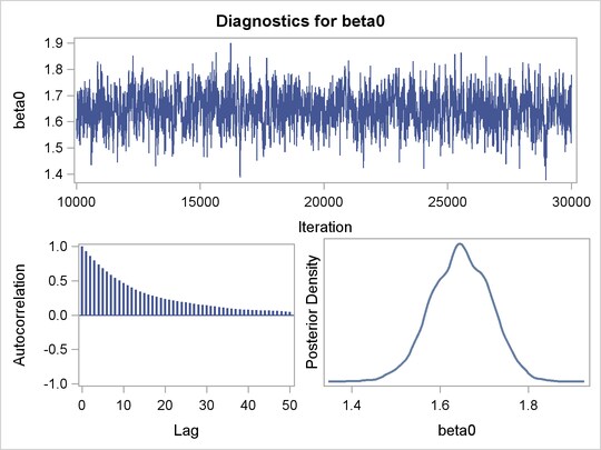
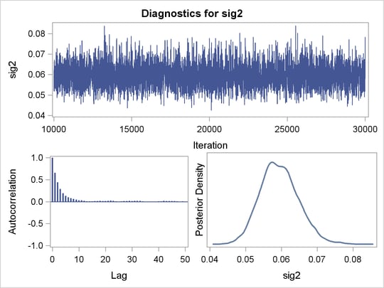
Figure 4
reports summary and interval statistics of all parameters. For example, the mean salary increases by an estimated factor of
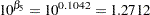 (approximately 27%) for each year the player was in Major League Baseball. Similarly, using the same formula,
 , you can see how the mean salary changes by one unit for each of the
covariates. Both the equal tail and highest posterior density (HPD) intervals include 0 for
, you can see how the mean salary changes by one unit for each of the
covariates. Both the equal tail and highest posterior density (HPD) intervals include 0 for
 , and
, and
 , indicating that the change in salary with respect to these covariates is not significant. The number of years played seems to be the most influential covariate, followed by the number of career hits.
Figure 4 Posterior Model Summary of Bayesian Linear Regression with Standardized Covariates
| Posterior Summaries | ||||||
|---|---|---|---|---|---|---|
| Parameter | N | Mean |
Standard
Deviation |
Percentiles | ||
| 25% | 50% | 75% | ||||
| beta0 | 20000 | 1.6465 | 0.0666 | 1.6006 | 1.6470 | 1.6935 |
| beta1 | 20000 | -0.00007 | 0.000938 | -0.00071 | -0.00004 | 0.000594 |
| beta2 | 20000 | 0.000882 | 0.00167 | -0.00023 | 0.000860 | 0.00200 |
| beta3 | 20000 | 0.00186 | 0.000993 | 0.00119 | 0.00186 | 0.00253 |
| beta4 | 20000 | 0.00218 | 0.000980 | 0.00152 | 0.00217 | 0.00281 |
| beta5 | 20000 | 0.1042 | 0.0205 | 0.0902 | 0.1038 | 0.1176 |
| beta6 | 20000 | 0.000748 | 0.000163 | 0.000642 | 0.000750 | 0.000857 |
| beta7 | 20000 | -0.00629 | 0.000978 | -0.00692 | -0.00629 | -0.00562 |
| beta8 | 20000 | -1.46E-7 | 5.867E-8 | -1.86E-7 | -1.47E-7 | -1.08E-7 |
| sig2 | 20000 | 0.0595 | 0.00533 | 0.0558 | 0.0592 | 0.0629 |
| Posterior Intervals | |||||
|---|---|---|---|---|---|
| Parameter | Alpha | Equal-Tail Interval | HPD Interval | ||
| beta0 | 0.050 | 1.5123 | 1.7714 | 1.5120 | 1.7705 |
| beta1 | 0.050 | -0.00195 | 0.00165 | -0.00192 | 0.00168 |
| beta2 | 0.050 | -0.00235 | 0.00417 | -0.00233 | 0.00418 |
| beta3 | 0.050 | -0.00006 | 0.00382 | -0.00001 | 0.00383 |
| beta4 | 0.050 | 0.000236 | 0.00412 | 0.000303 | 0.00416 |
| beta5 | 0.050 | 0.0651 | 0.1450 | 0.0625 | 0.1415 |
| beta6 | 0.050 | 0.000428 | 0.00107 | 0.000428 | 0.00107 |
| beta7 | 0.050 | -0.00827 | -0.00443 | -0.00822 | -0.00442 |
| beta8 | 0.050 | -2.62E-7 | -3.17E-8 | -2.63E-7 | -3.32E-8 |
| sig2 | 0.050 | 0.0498 | 0.0705 | 0.0494 | 0.0699 |
References
-
Mayer, L. S. and Younger, M. S. (1976), “Estimation of Standardized Regression Coefficients,” Journal of the American Statistical Association , 71(353), 154–157.
-
Reichler, J. L., ed. (1987), The 1987 Baseball Encyclopedia Update , New York: Macmillan.
-
Time Inc. (1987), “What They Make,” Sports Illustrated , 54–81.
These sample files and code examples are provided by SAS Institute Inc. "as is" without warranty of any kind, either express or implied, including but not limited to the implied warranties of merchantability and fitness for a particular purpose. Recipients acknowledge and agree that SAS Institute shall not be liable for any damages whatsoever arising out of their use of this material. In addition, SAS Institute will provide no support for the materials contained herein.
/*-----------------------------------------------------------------
  Example: Fitting a Bayesian Linear Regression model with
           Standardized Covariates
  Requires: SAS/STAT
  Version: 9.2
  ------------------------------------------------------------------*/

data baseball;
   input logSalary no_hits no_runs no_rbi no_bb yr_major cr_hits @@;
   yr_major2 = yr_major*yr_major;
   cr_hits2  = cr_hits*cr_hits;
   label no_hits="Hits in 1986" no_runs="Runs in 1986"
         no_rbi="RBIs in 1986"  no_bb="Walks in 1986"
         yr_major="Years in MLB" cr_hits="Career Hits"
         yr_major2="Years in MLB^2" cr_hits2="Career Hits^2"
         logSalary = "log10(Salary)";
   datalines;
           .  66 30 29 14  1   66
2.6766936096  81 24 38 39 14  835
2.6812412374 130 66 72 76  3  457
2.6989700043 141 65 78 37 11 1575
1.9614210941  87 39 42 30  2  101
2.8750612634 169 74 51 35 11 1133
  1.84509804  37 23  8 21  2   42
           2  73 24 24  7  3  108
1.8750612634 81 26 32 8 2 86
3.0413926852 92 49 66 65 13 1332
2.7136106505 159 107 75 59 10 1300
2.7096938697 53 31 26 27 9 467
2.7403626895 113 48 61 47 4 392
2.84509804 60 30 11 22 6 510
2.3802112417 43 29 27 30 13 825
. 39 20 15 11 3 42
2.8893017025 158 89 75 73 15 2273
2.2430380487 46 24 8 15 5 102
. 104 57 43 65 12 1478
2.1303337685 32 16 22 14 8 180
2 92 72 48 65 1 92
2.0606978404 109 55 43 62 1 109
. 98 48 49 43 15 1501
2.7781512504 116 60 62 74 6 489
2.8902348527 168 73 102 40 18 2464
2.8836614352 163 92 51 70 6 747
2.8502374753 73 32 18 22 7 491
2.8750612634 129 50 56 40 10 604
2.7958800173 152 92 37 81 5 633
2.9542425094 137 90 95 90 14 1382
. 84 42 30 39 17 1833
2.0413926852 108 55 36 22 3 149
. 141 70 87 52 9 994
2.787106093 168 83 80 56 5 452
2.4771212547 49 23 25 12 7 308
2.9294189257 106 38 60 30 14 1906
. 36 19 10 17 4 244
1.9542425094 60 24 25 15 2 78
. 98 31 53 30 16 1615
. 61 34 12 14 1 61
1.8293037728 41 15 21 33 2 50
. 54 21 18 15 18 1926
. 57 23 14 14 9 684
2.2552725051 46 32 19 9 4 160
. 40 19 29 30 11 1069
2.4842998393 68 28 26 22 6 236
2.3324384599 132 57 49 33 3 273
2.3935752033 57 34 32 9 5 192
. 140 46 75 41 16 2130
2.9111576087 146 71 70 84 6 715
2.942008053 101 42 63 22 17 1767
1.84509804 53 30 29 23 2 59
. 84 48 55 52 15 1016
3.079181246 168 80 72 39 9 1307
2.8293037728 101 45 53 39 12 1429
2.6180480967 102 49 85 20 6 231
2.531478917 58 28 25 35 4 333
. 61 24 39 21 14 1029
2.6197891057 78 32 41 12 12 968
3.1303337685 177 98 81 70 6 927
1.9542425094 113 58 69 16 1 113
2.4393326938 44 21 23 15 16 1634
2.361727836 56 27 15 11 4 270
2.3521825181 53 31 15 22 4 210
. 58 25 19 27 19 1981
2.9777236053 139 93 94 62 17 1982
. 37 12 17 14 4 163
1.8750612634 53 29 22 21 3 120
2.0211892991 142 67 86 45 4 205
. 113 44 27 44 12 1231
2.5051499783 81 42 30 26 17 2198
. 31 18 21 38 3 53
2.9294189257 131 69 96 52 14 1397
2.728353782 122 78 85 91 18 1947
2.9700366215 137 86 97 97 15 1785
2.9294189257 119 57 46 13 9 1046
2.3222192947 97 55 29 39 4 353
. 55 24 33 30 8 338
2.511883361 103 59 47 39 6 555
2.4393326938 96 37 29 23 4 290
. 118 70 94 33 16 1575
2.6532125138 70 49 35 43 15 1661
3.2955671 238 117 113 53 5 737
. 46 23 20 12 5 324
3.278753601 163 89 83 75 11 1388
2.7781512504 83 50 39 56 9 948
3.0177289059 174 89 116 56 14 2024
2.0413926852 82 44 45 47 2 113
2.414973348 41 21 29 22 16 1338
2.6766936096 114 67 57 48 4 298
2.6349808001 83 39 46 16 5 405
3.0863598307 123 76 93 72 4 471
1.84509804 78 35 35 32 1 78
2.1613680022 138 76 96 61 3 164
. 69 24 21 29 8 565
2.7745169657 119 54 58 36 12 594
3.2698537083 148 90 104 77 14 2083
. 71 27 29 14 15 1647
2.4771212547 115 97 71 68 3 184
2.69019608 110 70 47 36 7 544
3.3909351071 151 61 84 78 10 1679
. 132 69 47 54 2 260
2.5740312677 49 41 23 18 8 336
. 106 48 56 35 10 571
. 114 67 67 53 13 1632
. 37 15 19 15 6 244
. 95 55 58 37 3 139
2.8750612634 154 76 84 43 14 1583
3.0700378666 198 101 108 41 5 610
1.84509804 51 19 18 11 1 51
3.1760912591 128 70 73 80 14 2095
2.5854607295 76 33 52 37 5 351
3.2845595366 125 81 105 62 13 1646
2.3324384599 152 91 101 64 3 260
. 64 30 42 24 18 1925
2.9542425094 171 91 108 52 6 728
2.1903316982 118 63 54 30 4 187
2.84509804 77 45 47 26 16 1910
2.728353782 94 42 36 66 9 866
2.5593080109 85 30 44 20 8 568
2.8653012287 96 49 46 60 15 1972
2.3010299957 77 36 55 41 20 2172
2.6020599913 139 93 58 69 5 369
2.6020599913 84 62 33 47 5 376
2.8677620247 126 42 44 35 11 1578
. 59 45 36 58 13 1051
2.6989700043 78 37 51 29 5 453
2.7781512504 120 54 51 31 8 900
2.8211858826 158 70 84 42 5 636
2.9777236053 169 72 88 38 7 1077
2.8750612634 104 50 58 25 7 822
2.4734869701 54 30 39 31 5 299
2.511883361 70 22 37 18 18 2081
1.942008053 99 46 24 29 4 129
2.2430380487 39 18 30 15 9 151
1.9542425094 40 23 11 18 3 125
3.0925452076 170 107 108 69 6 634
2.6334684556 103 48 36 40 15 1193
. 69 33 18 25 5 361
2 103 65 32 71 2 103
2.2174839442 144 85 117 65 2 173
2.3979400087 200 108 121 32 4 404
3.1139433523 55 34 23 45 12 1213
2.888366543 133 48 72 55 17 2147
. 45 38 19 42 10 916
3.0036039807 132 61 74 41 6 671
2.4393326938 39 18 31 22 14 543
2.8893017025 183 80 74 32 5 715
2.9294189257 136 58 38 26 11 1066
2.5622928645 70 32 51 28 15 1130
. 61 32 26 26 11 408
1.9777236053 41 26 21 19 2 68
2.0413926852 86 33 38 45 1 86
2 95 48 42 20 10 808
2.4432629875 147 58 88 47 10 730
1.903089987 102 56 34 34 5 167
2.7781512504 94 37 32 26 13 1330
. 100 60 19 28 4 238
. 93 35 46 23 15 1610
2.3010299957 163 83 107 32 3 377
. 47 24 26 17 12 286
2.8175653696 174 67 78 58 6 880
1.8750612634 39 13 9 16 3 44
3.382467322 200 98 110 62 13 2163
2.3979400087 66 31 26 32 14 979
2.1903316982 76 35 60 25 3 151
2.806179974 157 90 78 26 4 541
2.4771212547 92 54 49 18 6 325
2.0413926852 73 23 37 16 4 108
. 69 32 19 20 4 209
2.9164539485 91 41 42 57 13 1397
. 54 28 44 18 2 59
2.2900346114 101 46 43 61 3 218
. 43 17 26 22 3 179
2.6532125138 47 20 28 18 11 890
2.7993405495 184 83 79 38 5 462
1.9370161075 58 34 23 22 1 58
3.1139433523 118 84 86 68 8 750
3 150 69 58 35 14 1839
3.2552725051 171 94 83 94 13 1840
3.1172712957 147 85 91 71 6 815
2.8677620247 74 34 29 22 10 1062
2.7958800173 161 89 96 66 4 470
2.096910013 91 51 43 33 2 94
3.0184229441 159 72 79 53 9 880
2.8603380066 136 62 48 83 10 970
2.4771212547 85 69 64 88 7 214
2.5622928645 223 119 96 34 3 587
1.8750612634 64 31 26 30 1 64
3.073106976 127 66 65 67 7 844
2.3064250276 127 77 45 58 2 187
2.3521825181 70 33 37 27 12 1222
2.7201593034 141 77 47 37 15 1240
2.4232458739 52 26 28 21 6 191
2.8962505625 149 89 86 64 7 928
2.903089987 84 53 62 38 10 1123
2.7690078709 128 67 94 52 13 1552
. 34 20 13 17 1 34
2.1613680022 92 42 60 21 3 185
. 146 80 44 46 9 915
2.6232492904 157 95 73 63 10 1320
1.8750612634 54 27 25 33 1 54
2.7596678447 179 94 60 65 5 476
. 53 18 26 27 4 228
2.8920946027 131 77 55 34 7 549
1.9542425094 56 22 36 19 2 58
2.1760912591 93 47 30 30 2 230
2.84509804 148 64 78 49 13 1000
. 59 20 37 27 4 209
2.7403626895 131 68 77 33 6 398
. 88 40 32 19 8 715
2.8129133566 65 30 36 27 9 698
1.8325089127 54 25 14 12 1 54
2 71 18 30 36 3 76
2.8260748027 77 47 53 27 6 516
2.2430380487 120 71 71 54 3 259
2.1367205672 60 28 33 18 3 170
3.3278354771 160 97 119 89 15 1954
2.942008053 94 36 26 62 7 519
2.079181246 43 26 35 39 3 116
2.1461280357 75 38 23 26 3 160
2.3222192947 167 89 49 57 4 232
2.903089987 110 61 45 32 7 834
2.3802112417 76 34 37 15 4 408
2.5440680444 93 43 42 49 5 323
. 76 35 41 47 4 326
2.2430380487 137 58 47 12 2 271
2.3010299957 152 105 49 65 2 249
. 84 46 27 21 12 1257
3.2878017299 144 67 54 79 9 1169
2.84509804 80 45 48 63 7 359
2.8750612634 163 88 50 77 4 470
2.6532125138 83 43 41 30 14 1543
2.2355284469 135 82 88 55 1 135
3.1003705451 123 62 55 40 9 1203
. 160 86 90 87 5 602
2.278753601 56 41 19 21 5 329
2.7634279936 154 61 48 29 6 566
2.1139433523 72 33 31 26 5 82
2.6532125138 77 35 29 33 12 1358
2.4771212547 96 50 45 39 5 344
2.3979400087 56 22 18 15 12 665
3.0211892991 70 42 36 44 16 1845
2.3324384599 108 75 86 72 3 142
2.6020599913 68 42 29 45 18 939
. 119 49 65 37 7 583
2.748188027 110 45 49 46 9 658
3.2227164711 160 130 74 89 8 1182
2.68797462 101 65 58 92 20 2510
. 90 73 49 64 11 1056
2.6283889301 82 42 60 35 5 408
2.6989700043 145 51 76 40 11 1102
. 44 28 16 11 1 44
. 80 42 36 29 7 656
2.3979400087 76 35 39 13 6 234
2.6020599913 52 31 27 17 12 1323
2.6532125138 90 50 45 43 10 614
2.8750612634 135 52 44 52 9 895
1.84509804 68 32 22 24 1 68
2.942008053 119 57 33 21 7 882
2.278753601 108 63 48 40 4 278
2.2810333672 68 42 42 61 6 238
2.8692317197 178 68 76 46 6 902
2.3979400087 86 38 28 36 4 267
2.1461280357 57 32 25 18 3 170
1.9890046157 101 50 55 22 1 101
2.8692317197 113 59 57 68 12 1369
2.1461280357 149 73 47 42 1 149
2.5336030344 63 25 33 16 10 667
. 84 35 32 23 2 87
3 163 82 46 62 13 2019
2 117 54 88 43 6 412
1.9542425094 66 20 28 13 3 80
2.3010299957 140 73 77 60 4 185
2.1303337685 112 54 54 35 2 160
2.1903316982 145 66 68 21 2 210
2.6766936096 159 82 50 47 6 426
3.1613680022 142 58 81 23 18 2583
2.1760912591 96 44 36 65 4 148
2.0211892991 103 53 33 52 2 123
2.5440680444 122 67 45 51 4 403
1.9542425094 210 91 56 59 6 872
. 112 40 58 24 11 1134
2.7242758696 169 88 73 53 8 841
2.5336030344 76 42 25 20 8 657
2.9731278536 152 69 75 53 6 686
2.5440680444 213 91 65 27 4 448
2.5141052641 103 48 28 54 8 493
2.3979400087 70 26 23 30 4 220
2.8692317197 211 107 59 52 5 770
2.6283889301 68 26 30 29 7 339
. 63 36 41 44 17 1954
2.9661417327 141 48 61 73 8 874
2.2671717284 120 53 44 21 4 227
2.9637878273 114 46 57 37 9 916
2.4573777015 43 24 17 20 7 219
2.3891660844 47 21 29 24 6 256
. 46 19 18 17 5 238
2.3710678623 61 17 22 3 17 1145
3.0606978404 147 56 52 53 7 821
2.2041199827 138 56 59 34 3 357
. 51 14 29 25 23 2732
2.6283889301 113 76 52 76 5 397
2.9542425094 42 17 14 15 10 1150
. 194 91 62 78 8 1028
2.6989700043 32 14 25 12 19 2402
2.4432629875 69 35 31 32 4 355
2.8750612634 112 50 71 44 7 771
2.2041199827 139 94 29 60 2 309
3.1139433523 186 107 98 74 6 753
2.7201593034 81 37 44 37 7 566
2.7403626895 124 67 27 36 7 506
3.2041199827 207 107 71 105 5 978
2.079181246 117 66 41 34 1 117
2.2174839442 172 82 100 57 1  172
           .  53 21 23 22  8  283
  2.84509804 127 65 48 37  5  806
 2.942008053 136 76 50 94 12 1511
2.5854607295 126 61 43 52  6  433
 2.982271233 144 85 60 78  8  857
           3 170 77 44 31 11 1457
;


proc means data = baseball mean stddev;
   output out=sum_baseball(drop=_type_ _freq_);
run;

ods graphics on;
proc mcmc data=baseball nbi=50000 nmc=10000 seed=1181 propcov=quanew;
   array beta[9] beta0-beta8;
   array data[9] 1 no_hits  no_runs  no_rbi no_bb
      yr_major cr_hits yr_major2 cr_hits2;

   parms beta: 0;
   parms sig2 1;

   prior beta: ~ normal(0,var = 1000);
   prior sig2 ~ igamma(shape = 3/10, scale = 10/3);

   call mult(beta, data, mu);
   model logsalary ~ n(mu, var = sig2);
run;
ods graphics off;

proc transpose data=sum_baseball out=tab;
   id _stat_;
run;

data _null_;
   set tab;
   sub = put((_n_-1), 1.);
   call symputx(compress('m' || sub,'*'), mean);
   call symputx(compress('s' || sub,'*'), std);
run;

%put &m1 &m2 &m3 &m4 &m5 &m6 &m7 &m8;
%put &s1 &s2 &s3 &s4 &s5 &s6 &s7 &s8;

proc standard data=baseball out=baseball_std mean=0 std=1;
   var no_hits -- cr_hits2;
run;

ods graphics on;
proc mcmc data=baseball_std nbi=10000 nmc=20000 seed=1181
   propcov=quanew monitor=(beta0-beta8 sig2);
   array beta[9] beta0-beta8 (0);
   array betastar[9] betastar0-betastar8;
   array data[9] 1 no_hits  no_runs  no_rbi no_bb
      yr_major cr_hits yr_major2 cr_hits2;
   array mn[9] (0 &m1 &m2 &m3 &m4 &m5 &m6 &m7 &m8);
   array std[9] (0 &s1 &s2 &s3 &s4 &s5 &s6 &s7 &s8);

   parms betastar: 0;
   parms sig2 1;

   prior betastar: ~ normal(0,var = 1000);
   prior sig2 ~ igamma(shape = 3/10, scale = 10/3);

   call mult(betastar, data, mu);
   model logsalary ~ n(mu, var = sig2);

   beginprior;
      summ = 0;
      do i = 2 to 9;
         beta[i] = betastar[i]/std[i];
         summ = summ + beta[i]*mn[i];
      end;
      beta0 = betastar0 - summ;
   endprior;
run;
ods graphics off;
These sample files and code examples are provided by SAS Institute Inc. "as is" without warranty of any kind, either express or implied, including but not limited to the implied warranties of merchantability and fitness for a particular purpose. Recipients acknowledge and agree that SAS Institute shall not be liable for any damages whatsoever arising out of their use of this material. In addition, SAS Institute will provide no support for the materials contained herein.
| Type: | Sample |
| Topic: | Analytics ==> Bayesian Analysis SAS Reference ==> Procedures ==> MCMC |
| Date Modified: | 2016-10-17 13:33:46 |
| Date Created: | 2012-02-03 10:49:33 |
Operating System and Release Information
| Product Family | Product | Host | Product Release | SAS Release | ||
| Starting | Ending | Starting | Ending | |||
| SAS System | SAS/STAT | Windows 7 Professional 32 bit | 9.3 | |||
| Windows 7 Home Premium x64 | 9.3 | |||||
| Windows 7 Home Premium 32 bit | 9.3 | |||||
| Windows 7 Enterprise x64 | 9.3 | |||||
| Windows 7 Enterprise 32 bit | 9.3 | |||||
| Microsoft Windows XP Professional | 9.3 | |||||
| Microsoft Windows Server 2008 | 9.3 | |||||
| Microsoft Windows Server 2008 for x64 | 9.3 | |||||
| Microsoft Windows Server 2003 for x64 | 9.3 | |||||
| Microsoft Windows Server 2003 Standard Edition | 9.3 | |||||
| Microsoft Windows Server 2003 Enterprise Edition | 9.3 | |||||
| Microsoft Windows Server 2003 Datacenter Edition | 9.3 | |||||
| Microsoft Windows NT Workstation | 9.3 | |||||
| Microsoft Windows 2000 Professional | 9.3 | |||||
| Microsoft Windows 2000 Server | 9.3 | |||||
| Microsoft Windows 2000 Datacenter Server | 9.3 | |||||
| Microsoft Windows 2000 Advanced Server | 9.3 | |||||
| Microsoft Windows 95/98 | 9.3 | |||||
| Microsoft® Windows® for x64 | 9.3 | |||||
| z/OS | 9.3 | |||||
| Windows 7 Professional x64 | 9.3 | |||||
| Windows 7 Ultimate 32 bit | 9.3 | |||||
| Windows 7 Ultimate x64 | 9.3 | |||||
| Windows Millennium Edition (Me) | 9.3 | |||||
| Windows Vista | 9.3 | |||||
| Windows Vista for x64 | 9.3 | |||||
| 64-bit Enabled AIX | 9.3 | |||||
| 64-bit Enabled HP-UX | 9.3 | |||||
| 64-bit Enabled Solaris | 9.3 | |||||
| HP-UX IPF | 9.3 | |||||
| Linux | 9.3 | |||||
| Linux for x64 | 9.3 | |||||
| Solaris for x64 | 9.3 | |||||