Binary Probit/Logit Regression Task
About the Binary Probit/Logit Regression Task
The Binary Probit/Logit
Regression task performs a regression analysis of a binary dependent
variable from normal or logistic distributed panel data.
Note: The version of the task depends
on what version of SAS/ETS is available at your site. For example,
if your site is running the second maintenance release for SAS 9.3,
SAS/ETS 12.1 is available, and SAS Studio is running version 1 of
the Binary Probit/Logit Regression task. If your site is running SAS
9.4, SAS/ETS 12.3 or later is available, and SAS Studio is running
version 2 of the Binary Probit/Logit Regression task. The difference
between the two versions is the addition of new options in SAS/ETS
12.3 or later.
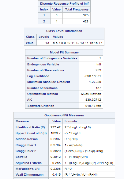
Example: Binary Probit/Logit Regression Task
To create this example:
-
Create the Work.Mroz data set. For more information, see MROZ Data Set.

Assigning Data to Roles
To run the Binary Probit/Logit
Regression task, you must assign a column to the Dependent
variable role.
|
Role
|
Description
|
|---|---|
|
Dependent
variable
|
specifies the numeric
column to use as the dependent variable for the regression analysis.
Use the Distribution drop-down
list to specify whether to create a normal or logistic model.
|
|
Continuous
variables
|
specifies the numeric
columns to use as the independent regressor (explanatory) variables
for the regression model.
|
|
Categorical
variables
|
specifies how to group
values into levels.
|
Setting Options
|
Option
|
Description
|
|---|---|
|
Methods
|
|
|
Type of
covariances of the parameter estimates
|
specifies the type of
covariance matrix of the parameter estimates.
You can specify these
types of matrices:
|
|
Include
the intercept in the model
|
specifies whether to
include the intercept in the model.
|
|
Heteroscedasticity
|
|
|
Analyze
heteroscedasticity
|
displays the heteroscedasticity
options.
|
|
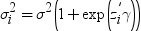
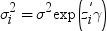
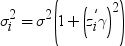
Variables
on the variance function
|
specifies the columns
that are related to heteroscedasticity of the residuals and how these
variables are used to model error variances. Here is the heteroscedastic
regression model that is supported by this task:
 |
|
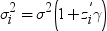
Form of
variance function
|
specifies the link function
to use. You can choose from these options:
|
|
Optimization
|
|
|
Method
|
specifies the iterative
minimization method to use. By default, the Quasi-Newton method is
used.
|
|
Maximum
number of iterations
|
specifies the maximum
number of iterations for the selected method.
|
|
Statistics
|
|
|
You can specify whether
to include any statistics in the results.
Here is the information
that you can choose to include in the results:
|
|
|
Plots
|
|
|
Select plots
to display
|
specifies whether to
display the default plots created by the task, only the plots that
you select, or no plots.
|
|
Diagnostic Plots
|
|
|
Error standard
deviations by observed regressor
|
displays the error standard
deviation versus observed regressors when you assign a column to the Variables
on the variance function option.
|
|
Profiled
log likelihood
|
displays the profiled
log likelihood. Each profiled graph is obtained by setting all the
parameters to their maximum likelihood estimate except for the profiling
parameter. The profiling parameter takes values on a predefined grid
that is determined by the maximum likelihood estimate of the corresponding
standard deviation.
|
|
Output Plots
|
|
|
Predicted
values by regressor
|
displays the model predicted
values. Each contributing regressor is set equal to its mean, except
for the parameter that is reported on the X axis.
|
|
Marginal
effects by regressor
|
displays the marginal
effects. Each contributing regressor is set equal to its mean, except
for the parameter that is reported on the X axis.
|
|
Inverse
Mills ratio by regressor
|
displays the inverse
Mills ratio. Each contributing regressor is set equal to its mean,
except for the parameter that is reported on the X axis.
|
|
Predicted
response probability by regressor
|
displays the predicted
response probability. Each contributing regressor is set equal to
its mean, except for the parameter that is reported on the X axis.
|
|
Predicted
probabilities for each level of the response by regressor
|
displays the predicted
probabilities for each level of the response. Each contributing regressor
is set equal to its mean, except for the parameter that is reported
on the X axis.
|
|
Linear predictor
values by regressor
|
displays the structural
part on the right side of the model. Each contributing regressor is
set equal to its mean, except for the parameter that is reported on
the X axis.
|
|
Display
as
|
specifies whether to
display the plots in a panel or individually.
|
Copyright © SAS Institute Inc. All rights reserved.