Summary Statistics Task

About the Summary Statistics Task

The Summary Statistics task provides data summarization tools to compute descriptive statistics for variables across all observations and within groups of observations. You can also summarize your data in a graphical display, such as a histogram.

For example, you could use this task to create a report on the number of new sales, arranged by product type and country.

Example: Summary Statistics of Unit Sales

In this example, you want to analyze unit sales. In addition to the tabular results, you choose to display a histogram of the distribution.

To create this example:

In the Tasks section, expand the Statistics folder and double-click Summary Statistics. The user interface for the Summary Statistics task opens.
On the Data tab, select the SASHELP.PRICEDATA data set.
To the Analysis variables role, assign the sale column.
On the Options tab, expand the Plots section and select the Histogram check box.
To run the task, click .

Here are the results:

Results from the MEAN and UNIVARIATE Procedures for Unit Sales

Assigning Data to Roles

To run the Summary Statistics task, you must assign a column to the Analysis variables role.

Role	Description
Roles
Analysis variables	The variables that you assign to this role are the numeric variables for which you want statistics. You must assign at least one variable to this role.
Classification variables	The variables that you assign to this role are character or discrete numeric variables that are used to divide the input data into categories or subgroups. The statistics are calculated on all selected analysis variables for each unique combination of classification variables.
Additional Roles
Group analysis by	The variables that you assign to this role are used to compute separate statistics for each distinct value or combination of values of the Group analysis by variables. The data is automatically sorted by the variables in this role before the statistics are computed.
Frequency count	When you assign a variable to this role, each observation in the table is assumed to represent n observations, where n is the value of the frequency count for that row. Statistics are calculated accordingly. You can assign a maximum of one variable to this role.
Weight variable	If you assign a variable to this role, the value of the variable for each observation is used to calculate weighted means, variances, and sums. You can assign a maximum of one variable to this role.

Setting Options

Option Name	Description
Basic Statistics
Mean	is the arithmetic average, calculated by adding the values of an analysis variable and dividing this sum by the number of nonmissing observations.
Standard deviation	is a statistical measure of the variability of a group of data values. This measure, which is the most widely used measure of the dispersion of a frequency distribution, is equal to the positive square root of the variance.
Minimum value	is the smallest value for an analysis variable.
Maximum value	is the largest value for an analysis variable.
Median	is the middle value for an analysis variable.
Number of observations	is the total number of observations with nonmissing values.
Number of missing values	is the number of observations with missing values.
Additional Statistics
Standard error	is the standard deviation of the sample mean. The standard error is defined as the ratio of the sample standard deviation to the square root of the sample size. Note: This option is available only if Degrees of freedom is selected in the Divisor for standard deviation and variance drop-down list.
Variance	is a statistical measure of dispersion of data values. This measure is an average of the total squared dispersion between each observation and the sample mean.
Mode	is the most frequent value for the analysis variable.
Range	is the difference between the largest and the smallest values in the data.
Sum	is the sum of all values in the analysis variable.
Sum of weights	is the sum of the numeric variable that is used to weight each observation. Note: You cannot compute the sum of the weights unless you assign a variable to the Weight variable role.
Confidence limits for the mean	are the two-sided confidence limits for the mean. A two-sided confidence interval for the mean has the following upper and lower limits: 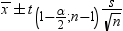$x with macron above , plus minus . t sub open 1 minus , alpha over 2 , semicolon n minus 1 close end sub . fraction s , over square root of n end fraction$ , where s is 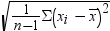$square root of fraction 1 , over n minus 1 end fraction . cap sigma . open , x sub i , minus , x with macron above , close squared end root$ and is the of the Student’s t statistics with degrees of freedom.
Coefficient of variation	is a unitless measure of relative variability. This measure is defined as the ratio of the standard deviation to the mean expressed as a percentage. The coefficient of variation is meaningful only if the variable is measured on a ratio scale.
Skewness	is skewness, which measures the tendency of the deviations to be larger in one direction than in the other.
Kurtosis	is the kurtosis, which measures the heaviness of tails.
Percentile Statistics
1st, 5th, 10th, Lower quartile, Median, Upper quartile, 90th, 95th, 99th, Interquartile range	choose the percentiles and quantiles to compute.
Quantile method	specifies the method that is used to compute the quantiles, median, and percentiles. Order statistics reads all of the data into memory and sorts it by the unique values. Piecewise-parabolic algorithm approximates the quantile and is a less memory-intensive method.
Plots
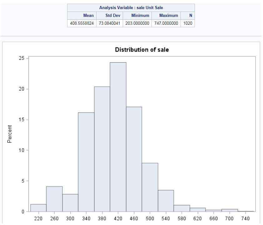
Histogram	creates a graph that is used to determine the distribution of the data. If you add a normal density curve, the task uses the sample mean and sample standard deviation for and . If you add a kernel density curve, the task uses the AMISE method to compute the kernel density estimates. To include the statistics in the graph, select the Add inset statistics check box.
Comparative box plot	creates a graph that shows a measure of central location (the median), two measures of dispersion (the range and interquartile range), the skewness (from the orientation of the median relative to the quartiles), and potential outliers. Box plots are especially useful in comparing two or more sets of data. Note: The Comparative box plot option is available only when no column is assigned to the Classification variable role. You can choose to add the overall inset statistics to the graph or only the inset statistics for each group.
Combine histogram and box plot	displays the histogram and box plots together in a single panel, sharing common X axes. You can choose to add the overall inset statistics to the graph. Note: The Combine histogram and box plot option is available only when no column is assigned to the Classification variable role.
Details
Divisor for standard deviation and variance	specifies the divisor to use in the calculation of the variance and standard deviation. Here are the valid options: Degrees of freedom By default, the divisor for the variance is the degrees of freedom. Number of observations n Sum of weights minus one Sum of weights
Output Data Set
You can specify whether to save the statistics in an output data set. By default, this data set is saved in the Work library.