Generalized Linear Models

About the Generalized Linear Models Task

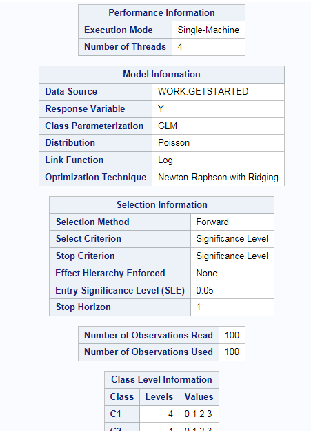
The Generalized Linear Models task is a high-performance task that provides model fitting and model building for generalized linear models. It fits models for standard distributions such as normal, Poisson, and Tweedie in the exponential family. This task also fits multinomial models for ordinal and nominal responses. The task provides forward, backward, and stepwise selection methods.

Note: This task is available only if you are running SAS 9.4.

Example: Model Selection

To create this example:

Create the Work.getStarted data set. For more information, see GETSTARTED Data Set.
In the Tasks section, expand the High Performance folder and double-click Generalized Linear Models. The user interface for the Generalized Linear Models task opens.
On the Data tab, select the WORK.GETSTARTED data set.

Assign columns to these roles:

Role	Description
Response variable	Y From the Distribution drop-down list, select Poisson.
Classification variables	C1 C2 C3 C4 C5

Click the Models tab. From the Selection method drop-down list under the Model Selection heading, select Forward selection.
To run the task, click .

Here is a subset of the results:

Performance Information, Model Information, Selection Information, and Class Level Information

Assigning Data to Roles

To run the Generalized Linear Model task, you must assign a column to the Response variable role.

Role	Description
Roles
Response variable	specifies the numeric column that contains the count values. The dependent count variable should be only nonnegative integer values in the input data set. You can specify these distributions for your model: Binary Gamma Inverse Gaussian Multinomial Negative binomial Normal Poisson You can specify these link functions for your model: complementary log-log log-log logit generalized logit probit identity reciprocal reciprocal square logarithm
Response variables (continued)	If you select Default for the link function, then the default link function for the model distribution is used. Here is the list of distributions with the corresponding default link function: Binomial distribution uses the logit link function. Gamma distribution uses the reciprocal link function. Inverse Gaussian distribution uses the reciprocal square link function. Multinomial distribution uses the cumulative logit link function. Negative binomial distribution uses the log link function. Normal distribution uses the identity link function. Poisson distribution uses the log link function.
Continuous variables	specifies the independent covariates (regressors) for the regression model. If you do not specify a continuous variable, the task fits a model that contains only an intercept.
Classification variables	specifies the variables to use to group (classify) data in the analysis. Classification variables can be either character or numeric.
Additional Roles
Frequency count	specifies the numeric column that contains the frequency of occurrence for each observation.
Weight variable	specifies the column to use as a weight to perform a weighted analysis of the data.

Building a Model

Requirements for Building a Model

By default, no effects are specified, which results in the task fitting an intercept-only model. To specify an effect, you must assign at least one variable to the Continuous variables or Classification variables role. You can select combinations of variables to create crossed, factorial, or polynomial effects.

Create a Main Effect

Select the variable name in the Variables box.
Click Add to add the variable to the Model effects box.

Create Crossed Effects (Interactions)

Select two or more variables in the Variables box. To select more than one variable, press Ctrl.
Click Cross.

Create a Two-Way Factorial Model

Select two or more variables in the Variables box.
Click Two-way Factorial.

For example, if you select the Height, Weight, and Age variables and then click Two-way Factorial, these model effects are created: Age, Height, Weight, Age*Height, Age*Weight, and Height*Weight*Age.

Create a Full Factorial Model

Select two or more variables in the Variables box.
Click Full Factorial.

For example, if you select the Height, Weight, and Age variables and then click Full Factorial, these model effects are created: Age, Height, Weight, Age*Height, Age*Weight, Height*Weight, and Age*Height*Weight.

Create N-Way Factorial

Select two or more variables in the Variables box.
Click N-way Factorial to add these effects to the Model effects box.

For example, if you select the Height, Weight, and Age variables and then specify the value of N as 3, when you click N-way Factorial, these model effects are created: Age, Height, Weight, Age*Height, Age*Weight, Height*Weight, and Age*Height*Weight.

Create Polynomial Effects

Select one variable in the Variables box.
Specify higher-degree crossings by adjusting the number in the N field.
Click Polynomial, Degree=N to add the polynomial effects to the Model effects box.

Create Polynomial Effects of the N Order

Select one variable in the Variables box.
Specify higher-degree crossings by adjusting the number in the N field.
Click Polynomial, Order=N to add the polynomial effects to the Model effects box.

For example, if you select the Age and Height variables and then you specify 3 in the N field, when you click Polynomial, Order=N, these model effects are created: Age, Age*Age, Age*Age*Age, Height, Height*Height, and Height*Height*Height.

Setting the Model Options

Option	Description
Model
Include an intercept in the model	specifies whether to include the intercept in the model.
Offset variable	specifies a variable to be used as an offset to the linear predictor. An offset plays the role of an effect whose coefficient is known to be 1. Observations that have missing values for the offset variable are excluded from the analysis.
Model Selection
Selection method	specifies the model selection method for the model. The task performs model selection by examining whether effects should be added to or removed from the model according to the rules that are defined by the selection method. Here are the valid values for the selection methods: None fits the full model. Forward selection started with no effects in the model and adds effects based on the Significance level to add an effect to the model option. Backward elimination starts with all the effects in the model and deletes effects based on the value in the Significance level to remove an effect from the model option. Stepwise regression is similar to the forward selection model. However, effects that are already in the model do not necessarily stay there. Effects are added to the model based on the Significance level to add an effect to the model option and are removed from the model based on the Significance level to remove an effect from the model option.
Select best model by	specifies what criterion to use to select the best model.

Setting Options

Option	Description
Tables
You can specify whether to include any output tables in the results. Here are the additional tables that you can include: Confidence limits for estimates Correlations of parameter estimates Covariances of parameter estimates
Output Data Set
You can specify whether to create an output data set. By default, the data set is saved in the Work library. In the output, you can also include these statistics: linear predictors predicted values lower confidence limit for predicted values upper confidence limit for predicted values residuals Pearson residuals adjusted Pearson residuals You can also select any columns from the input data set to include in the output data.
Optimization
Method	specifies the optimization technique to use.
Maximum number of iterations	specifies the maximum number of iterations to perform for the selected optimization technique.