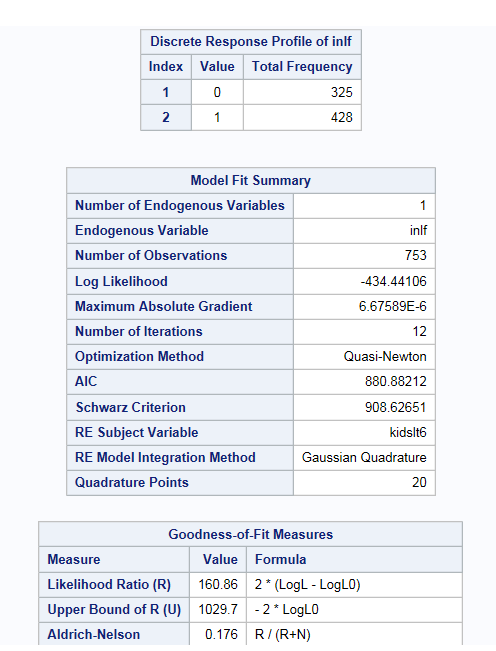
Probit Model :: SAS(R) Studio 3.5: Task Reference Guide

Example: Probit Model

To create this example:

Create the Work.Moz data set. For more information, see MROZ Data Set.
In the Tasks section, expand the Econometrics folder, and then double-click Panel Data Models. The user interface for the Panel Data Models task opens.
On the Data tab, select the WORK.MROZ data set.

Tip
If the data set is not available from the drop-down list, click . In the Choose a Table window, expand the library that contains the data set that you want to use. Select the data set for the example and click OK. The selected data set should now appear in the drop-down list.

Assign columns to these roles:

Role	Column Name
Panel Structure
Cross-sectional ID	kidslt6
Roles
Dependent variable	inlf
Continuous variables	nwifeinc educ exper expersq
Categorical variable	kidsge6

On the Model tab, select Probit as the model type.
To run the task, click .

Here is a subset of the results:

Assigning Data to Roles

To perform an analysis of a probit model, you must assign an input data set. To filter the input data source, click Filter Icon

.

You also must assign variables to the Cross-sectional ID and Dependent variable roles.

Role	Description
Panel Structure
Cross-sectional ID	specifies the cross section for each observation. The task verifies that the input data is sorted by the cross-sectional ID. Note: For the probit model, character variables are not supported.
Time ID	specifies the time period for each observation. For each cross section, the values of the time ID must be unique. Note: For the probit model, a time ID is not required and is ignored in the analysis.
Roles
Dependent variable	specifies the numeric variable that takes discrete values.
Continuous variables	specifies the independent covariates (regressors) for the regression model. If you do not specify a continuous variable, the task fits a model that contains only an intercept.
Categorical variables	specifies the classification variables. The task generates dummy variables for each level of the categorical variable.
Additional Roles
Group analysis by	enables you to obtain separate analyses of observations for each unique group.

Setting the Model Options

To create a probit model:

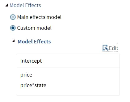
From the Model type drop-down list, select Probit.
Specify the model effects.
You can display the main effects model or create a custom model. To create a custom model, select the Custom Model option, and then click Edit. The Model Effects Builder opens. All continuous variables and categorical variables are listed in the Variables pane.
- To create a main effect, select the variable in the Variables pane, and then click Add.
- To create a crossed effect, select the variables in the Variables pane. (You can use Ctrl to select multiple variables.) Then click Cross.
When you finish, click OK. The effects that you specified now appear on the Model tab.

Here is an example of model effects on the Model tab.

Note: Random effects are automatically included in the model. This functionality is experimental.
Specify the threshold for the first category for the probit model. By default, this value is zero, but you can use an estimated value.

Setting the Options

Option Name	Description
Methods
Covariance matrix estimator	specifies the method to calculate the covariance matrix of parameter estimates. You can use the default method, or you can choose from these covariance types: Inverse Hessian matrix – the covariance from the inverse Hessian matrix. Outer product matrix – the covariance from the outer product matrix. Outer product and Hessian matrices – the covariance from the outer product and Hessian matrices (the quasi-maximum likelihood estimates).
Optimization
Method	specifies the optimization method to use.
Maximum number of iterations	specifies the maximum number of iterations in the optimization process. You can use the default value or specify a custom value.
Statistics
Select the statistics to display in the results. Here are the additional statistics that you can include in the results: correlations of the parameter estimates covariances of the parameter estimates iteration history of the objective function and parameter estimates
Plots
You can choose to display only the default plots, the selected plots, or no plots in the results. You can choose from these types of plots: diagnostic plots, such as error standard deviations by observed regressor and profiled log likelihood output plots, such as predicted values by regressor, marginal effects by regressor, Inverse Mills ratio by regressor, predicted response probability by regressor, predicted probabilities for each level of the response by regressor, and linear predictor values by regressor

Creating the Output Data Sets

You can create these output data sets:

an output data set that contains the default statistics from the analysis and additional statistics, such as predicted values, the probability of the dependent variable taking the current value, the probability of the dependent variable for all possible responses, and the error standard deviation
a parameter estimates data set