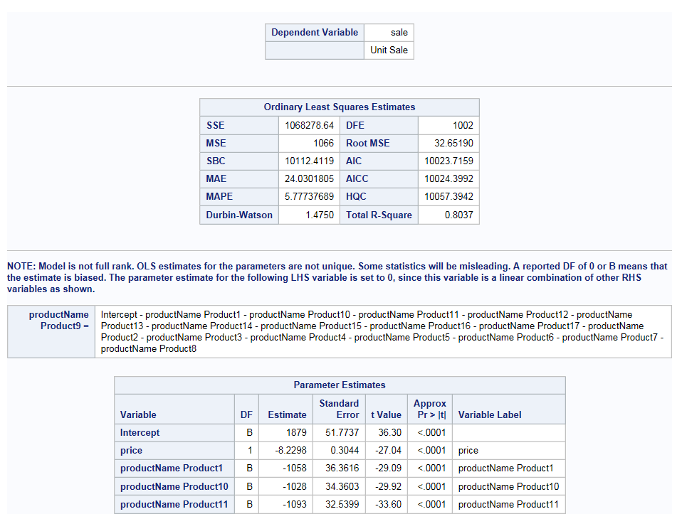
Time Series Analysis for One Dependent Variable :: SAS(R) Studio 3.5: Task Reference Guide

Example: Analyzing Sales Data

To create this example:

In the Tasks section, expand the Econometrics folder, and then double-click Time Series Analysis. The user interface for the Time Series Analysis task opens.
On the Data tab, select the SASHELP.PRICEDATA data set.

Tip
If the data set is not available from the drop-down list, click . In the Choose a Table window, expand the library that contains the data set that you want to use. Select the data set for the example and click OK. The selected data set should now appear in the drop-down list.

Assign columns to these roles:

Role	Column Name
Dependent variables	sale
Continuous variables	price
Categorical variables	productName

To run the task, click .

Here is a subset of the results:

Ordinary Least Squares Estimates and Parameter Estimates

Yule-Walker Estimates and Parameter Estimates

Assigning Data to Roles

To perform a time series analysis, you must assign an input data set. To filter the input data source, click Filter Icon

.

You also must assign a variable to the Dependent variables role.

Role	Description
Roles
Dependent variables	specifies the dependent variable for the analysis. Note: You can assign more than one dependent variable. The remaining task options differ slightly if you have multiple dependent variables. For more information, see Time Series Analysis for Multiple Dependent Variables.
Independent Variables
Continuous variables	specifies the independent variables for the model.
Categorical variables	specifies the classification variables to use in the analysis. The analysis produces a singular model.
Additional Roles
Group analysis by	specifies how to sort the data. Analyses are performed on each group. Note: This role is not available if you have a categorical variable.

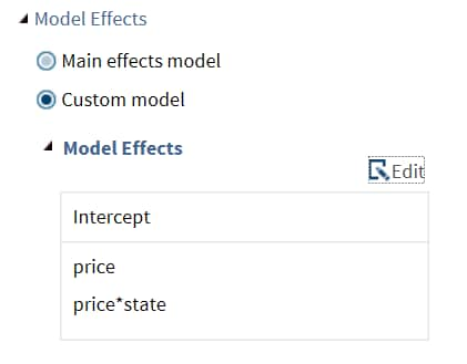
Setting the Model Options

You can display the main effects model or create a custom model. To create a custom model, select the Custom Model option, and then click Edit. The Model Effects Builder opens. All continuous variables and categorical variables are listed in the Variables pane.

To create a main effect, select the variable in the Variables pane, and then click Add.
To create a crossed effect, select the variables in the Variables pane. (You can use Ctrl to select multiple variables.) Then click Cross.

When you finish, click OK. The effects that you specified now appear on the Model tab.

Here is an example of model effects on the Model tab.

Here are the remaining options on the Model tab.

Option Name	Description
Error Model Options
Automatically select error process orders	removes insignificant autoregressive parameters. The parameters are removed in order of least significance.
Autoregressive order (p), Maximum autoregressive order (p)	specifies the order of the autoregressive error process.
Garch Conditional Heteroscedasticity
ARCH process order (q)	specifies the order of the process or the subset of ARCH terms to be fitted.
GARCH process order (p)	specifies the order of the process or the subset of GARCH terms to be fitted. Note: This option is available only if you specify the ARCH process order greater than 0.
GARCH model type	specifies the type of model. Here are the valid options: Exponential GARCH Power GARCH Quadratic GARCH Threshold GARCH GARCH with no constraints Note: This option is available only if you specify the ARCH process order greater than 0.

Setting the Options

Option Name	Description
Methods
Method	specifies the optimization method to use. By default, no optimization method is used.
Maximum number of iterations	specifies the maximum number of iterations. The default is 100 iterations.
Tests
Tests for Autocorrelation
Generalized Durbin-Watson test	runs the Durbin-Watson test for the first order.
Tests for Heteroscedasticity
specifies tests for the absence of ARCH effects. Here are the valid tests: Q and Engle’s LM tests Lee and King’s ARCH tests Wong and Li’s ARCH tests
Tests of Normality
Bera-Jarque normality test	specifies the Jarque-Bera’s normality test statistic for regression residuals.
Tests for Independence
specifies tests of independence. Here are the valid tests: Brock-Dechert-Scheinkman (BDS) test Runs test Turning point test Rank version of the von Neumann ratio test
Plots
You can choose to use the default results, include selected plots in the results, or include no plots in the results. You can also include these plots in the results: autocorrelation plot inverse-autocorrelations plot partial-autocorrelations plot Q-Q plot of residuals residuals studentized residuals standardized residuals white noise probabilities histogram of residuals

Creating an Output Data Set

You can create these output data sets:

an output data set that contains the predicted values, residuals, and confidence limits for the predictions
a parameter estimates data set