Using the Pivot By Feature

The pivot by feature provides an easy and powerful way to summarize data for analytics. You can specify a column to use as a categorical variable and the unique values to use. When the query is run, the output table is summarized with the aggregations that you apply.

To use the pivot by feature:

On the Column Editor tab, place your pointer in the Pivot By cell for the column to use as the pivot column. Click the ellipsis button to select the pivot column and values.
In the Pivot Values dialog box, select the pivot by column. You can enter search criteria in Filter fields to filter the column names.

The following display shows an example of pivoting by three values in the Product_Category column.

Pivot Values
After the unique values for the column are loaded, select the check boxes for the values to use in the summarization. Click Apply.

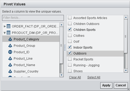
The following display shows an example of the Column Editor tab when a pivot by column is used. The minimum and maximum Total_Retail_Price are calculated for each Customer_ID and are then pivoted by (transposed by) three values of the Product_Category column.

Column Editor Tab with a Pivot By Column

Tip

TRP is specified as a label for the Total_Retail_Price column. Look at the next display to see how the label is used to create labels for the new columns.

The following display shows how pivoting the Customer_ID column by three values of the Product_Category column results in additional output columns. A substring of the pivot by values is used as a prefix to each column name and the aggregate function is used as a suffix. The pivot by column label and aggregate function are used in the output column label.

Output Columns Tab with Pivot By Values