Overview of Visualizations
Visualization Types
|
Automatically selects
the chart type according to the data that is assigned to the visualization.
When you are first exploring a new data set, autocharts are useful
to give you a quick view of the data.
For more information,
see Working with Automatic Charts.
|
||
|
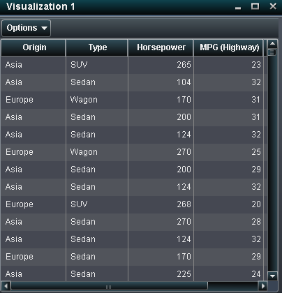
Displays the data as
a table. Tables enable you to examine the raw data for each observation
in the data source. You can rearrange the data columns and apply sorting.
For more information,
see Working with Tables.
|
||
|
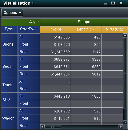
Displays the data as
a crosstab. Crosstabs enable you to examine the data for intersections
of category values. You can rearrange the rows and columns and apply
sorting.
For more information,
see Working with Crosstabs.
|
||
|
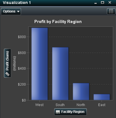
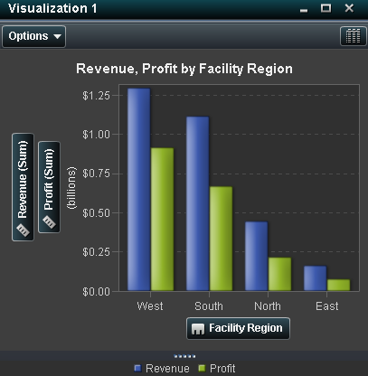
Displays the data as
a bar chart. Bar charts are especially useful for comparing data according
to each discrete value of a category.
You can configure a
bar chart with either vertical bars or horizontal bars. You can also
assign grouping to the bars and create lattices.
For more information,
see Working with Bar Charts.
|
||
|
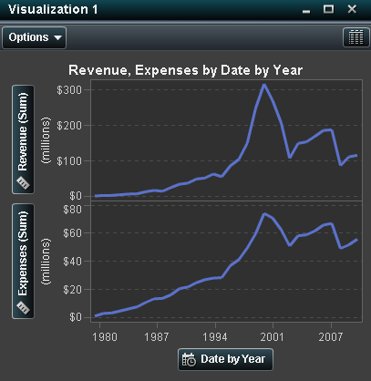
For more information,
see Working with Line Charts.
|
||
|
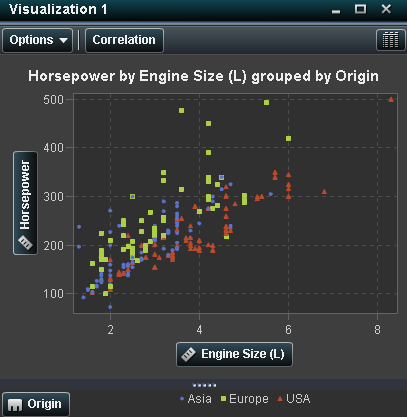
Displays the data as
a scatter plot. Scatter plots are most useful to examine the relationship
between variables.
In a scatter plot, you
can apply statistical analysis with correlation and regression. Scatter
plots also support grouping.
When you apply more
than two measures to a scatter plot, the visualization automatically
displays a scatter plot matrix to compare each pairing of measures.
For more information,
see Working with Scatter Plots.
|
||
|
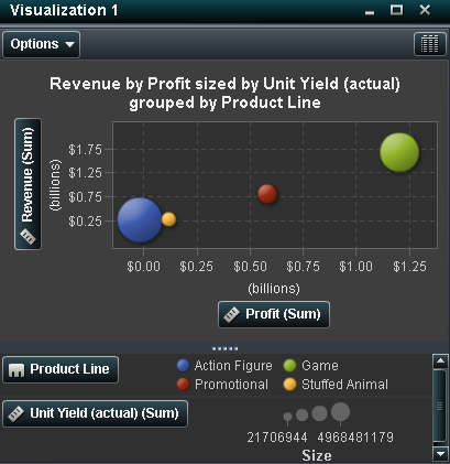
Displays the data as
a bubble plot. A bubble plot displays the relationship between three
measures, where two measures are represented by the plot axes and
the third measure is represented by the size of the plot markers.
You can apply grouping
and create lattices for a bubble plot. By assigning a datetime data
item to the plot, you can animate the bubbles to display changes in
the data over time.
For more information,
see Working with Bubble Plots.
|
||
|
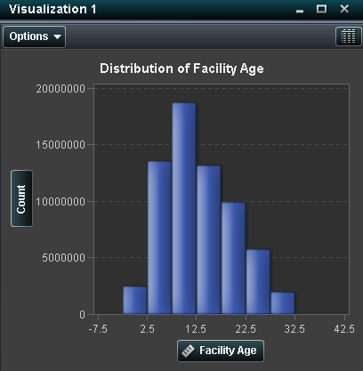
Displays the data as
a histogram. A histogram displays the distribution of values for a
single measure.
You can select the bar
orientation, and select whether the distribution values are displayed
as a percentage or as the row number of values.
For more information,
see Working with Histograms.
|
||
|
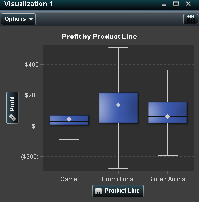
Displays the data as
a box plot. A box plot displays the distribution of values for a measure
by using a box. The size and location of the box indicate the range
of values that are between the 25th and 75th percentile. Additional
statistical information is represented by other visual features.
You can create lattices,
and select whether the average (mean) value and outliers are displayed
for each box.
For more information,
see Working with Box Plots.
|
||
|
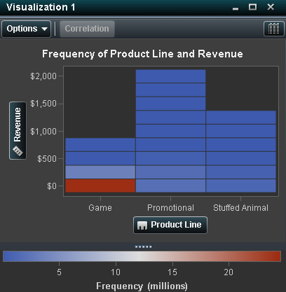
Displays the data as
a heat map. A heat map displays the distribution of values for two
data items by using a table with colored cells. If you do not assign
a measure to the color data role, then the cell colors represents
the frequency of each intersection of values. If you assign a measure
to the color data role, then the cell colors represent the measure
value for each intersection of values.
For more information,
see Working with Heat Maps.
|
||
|
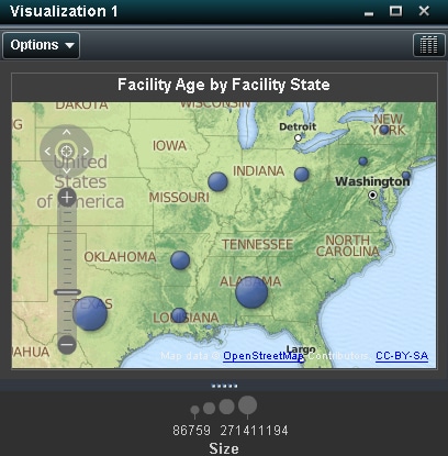
Displays the data as
a geo map. A geo map displays your data as a bubble plot that is overlaid
on a geographic map. Each bubble is located at a geographic location
or at the center of a geographical region.
For more information,
see Working with Geo Maps.
|
