ODS Graphics Template Modification

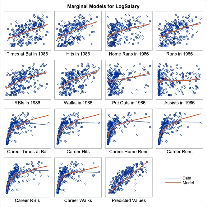
Marginal model plots (proposed by Cook and Weisberg 1997 and discussed by Fox and Weisberg 2011) display the marginal relationship between the response and each predictor. Marginal model plots display the dependent variable on each vertical axis and each independent variable on a horizontal axis. There is one marginal model plot for each independent variable and one additional plot that displays the predicted values on the horizontal axis. Each plot contains a scatter plot of the two variables, a smooth fit function for the variables in the plot (labeled "Data"), and a function that displays the predicted values as a function of the horizontal axis variable (labeled "Model"). (See Output 22.7.1.) When the two functions are similar in each of the graphs, there is evidence that the model fits well. When the two functions differ in at least one of the graphs, there is evidence that the model does not fit well. The two functions correspond well for some independent variables and deviate for others largely because of the outlier, Pete Rose, the career hits leader.

Marginal model plots provide useful diagnostic information for both linear and generalized linear models.You can use the %Marginal macro to produce marginal model plots after fitting a model. You must specify the dependent variable, the independent variables, and the variable that contains the predicted values. By default, the last SAS data set that is created is displayed, a loess fit function is used, and the macro chooses the number of graphs (from 2 to 15) to display in each panel and the size of the panel. Multiple panels are displayed when there are too many graphs to fit in a single panel. You can specify the number and size of the graphs in each panel rather than relying on the defaults.

The following steps illustrate the default settings:

%let vars =  nAtBat  nHits  nHome  nRuns  nRBI  nBB  nOuts nAssts
            CrAtBat CrHits CrHome CrRuns CrRbi CrBB;

proc glm noprint data=sashelp.baseball;
   class div;
   model logsalary = div &vars;
   output out=pvals p=p;
run; quit;

%marginal(independents=&vars, dependent=LogSalary, predicted=p)

Output 22.7.1 displays the results.