Introduction to Statistical Modeling with SAS/STAT Software
Univariate and Multivariate Models
A multivariate statistical model is a model in which multiple response variables are modeled jointly. Suppose, for example,
that your data consist of heights  and weights
  of children, collected over several years
  . The following separate regressions represent two univariate models:
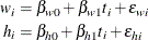
In the univariate setting, no information about the children’s heights "flows" to the model about their weights and vice versa. In a multivariate setting, the heights and weights would be modeled jointly. For example:
![\begin{align*} \bY _ i = \left[\begin{array}{ll} w_ i \cr h_ i \end{array}\right] & = \bX \bbeta + \left[\begin{array}{ll} \epsilon _{wi} \cr \epsilon _{hi} \end{array}\right] \\ & = \bX \bbeta + \bepsilon _ i \\ \bepsilon _ i & \sim \left(\mb{0}, \left[\begin{array}{cc} \sigma ^2_1 & \sigma _{12} \cr \sigma _{12} & \sigma ^2_2 \end{array}\right] \right) \end{align*}](images/statug_intromod0041.png)
The vectors  and
and  collect the responses and errors for the two observation that belong to the same subject. The errors from the same child
now have the correlation
collect the responses and errors for the two observation that belong to the same subject. The errors from the same child
now have the correlation
![\[ \mr{Corr}[\epsilon _{wi},\epsilon _{hi}] = \frac{\sigma _{12}}{\sqrt {\sigma ^2_1 \, \sigma ^2_2}} \]](images/statug_intromod0044.png)
and it is through this correlation that information about heights "flows" to the weights and vice versa. This simple example shows only one approach to modeling multivariate data, through the use of covariance structures. Other techniques involve seemingly unrelated regressions, systems of linear equations, and so on.
Multivariate data can be coarsely classified into three types. The response vectors of homogeneous multivariate data consist of observations of the same attribute. Such data are common in repeated measures experiments and longitudinal studies, where the same attribute is measured repeatedly over time. Homogeneous multivariate data also arise in spatial statistics where a set of geostatistical data is the incomplete observation of a single realization of a random experiment that generates a two-dimensional surface. One hundred measurements of soil electrical conductivity collected in a forest stand compose a single observation of a 100-dimensional homogeneous multivariate vector. Heterogeneous multivariate observations arise when the responses that are modeled jointly refer to different attributes, such as in the previous example of children’s weights and heights. There are two important subtypes of heterogeneous multivariate data. In homocatanomic multivariate data the observations come from the same distributional family. For example, the weights and heights might both be assumed to be normally distributed. With heterocatanomic multivariate data the observations can come from different distributional families. The following are examples of heterocatanomic multivariate data:
-
For each patient you observe blood pressure (a continuous outcome), the number of prior episodes of an illness (a count variable), and whether the patient has a history of diabetes in the family (a binary outcome). A multivariate model that models the three attributes jointly might assume a lognormal distribution for the blood pressure measurements, a Poisson distribution for the count variable and a Bernoulli distribution for the family history.
-
In a study of HIV/AIDS survival, you model jointly a patient’s CD4 cell count over time—itself a homogeneous multivariate outcome—and the survival of the patient (event-time data).