Introduction to Statistical Modeling with SAS/STAT Software
Linear and Nonlinear Models
A statistical estimation problem is nonlinear if the estimating equations—the equations whose solution yields the parameter estimates—depend on the parameters in a nonlinear fashion. Such estimation problems typically have no closed-form solution and must be solved by iterative, numerical techniques.
Nonlinearity in the mean function is often used to distinguish between linear and nonlinear models. A model has a nonlinear mean function if the derivative of the mean function with respect to the parameters depends on at least one other parameter. Consider, for example, the following models that relate a response variable Y to a single regressor variable x:
![\begin{align*} \mr{E}[Y|x] & = \beta _0 + \beta _1 x \\ \mr{E}[Y|x] & = \beta _0 + \beta _1 x + \beta _2 x^2 \\ \mr{E}[Y|x] & = \beta + x/\alpha \end{align*}](images/statug_intromod0015.png)
In these expressions, ![$\mr{E}[Y|x]$](images/statug_intromod0016.png) denotes the expected value of the response variable Y at the fixed value of x. (The conditioning on x simply indicates that the predictor variables are assumed to be non-random. Conditioning is often omitted for brevity in
this and subsequent chapters.)
denotes the expected value of the response variable Y at the fixed value of x. (The conditioning on x simply indicates that the predictor variables are assumed to be non-random. Conditioning is often omitted for brevity in
this and subsequent chapters.)
The first model in the previous list is a simple linear regression (SLR) model. It is linear in the parameters  and
and  since the model derivatives do not depend on unknowns:
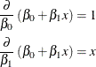
The model is also linear in its relationship with x (a straight line). The second model is also linear in the parameters, since
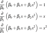
However, this second model is curvilinear, since it exhibits a curved relationship when plotted against x. The third model, finally, is a nonlinear model since
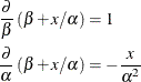
The second of these derivatives depends on a parameter  . A model is nonlinear if it is not linear in at least one parameter. Only the third model is a nonlinear model. A graph of
![$\mr{E}[Y]$](images/statug_intromod0023.png) versus the regressor variable thus does not indicate whether a model is nonlinear. A curvilinear relationship in this graph
can be achieved by a model that is linear in the parameters.
versus the regressor variable thus does not indicate whether a model is nonlinear. A curvilinear relationship in this graph
can be achieved by a model that is linear in the parameters.
Nonlinear mean functions lead to nonlinear estimation. It is important to note, however, that nonlinear estimation arises also because of the estimation principle or because the model structure contains nonlinearity in other parts, such as the covariance structure. For example, fitting a simple linear regression model by minimizing the sum of the absolute residuals leads to a nonlinear estimation problem despite the fact that the mean function is linear.