Shared Concepts and Topics
Truncated Power Function Basis
A truncated power function for a knot  is a function defined by
![\[ t_ i(x) = \left\{ \begin{array}{ll} 0 & \quad x<k_ i \\ (x-k_ i)^ d & \quad x\geq k_ i \end{array} \right. \]](images/statug_introcom0045.png)
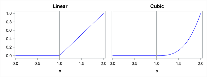
Figure 19.1 shows such functions for d = 1 and d = 3 with a knot at x = 1.
Figure 19.1: Truncated Power Functions with Knot at x = 1

The name is derived from the fact that these functions are shifted power functions that get truncated to zero to the left
of the knot. These functions are piecewise polynomial functions with two pieces whose function values and derivatives of all
orders up to  are zero at the defining knot. Hence these functions are splines of degree d. It is easy to see that these n functions are linearly independent. However, they do not form a basis, because such a basis requires
  functions. The usual way to add
  additional basis functions is to use the polynomials
  . These
  functions together with the n truncated power functions
  form the truncated power basis.
Note that each time a knot is repeated, the associated exponent used in the corresponding basis function is reduced by 1.
For example, for splines of degree d with three repeated knots  the corresponding basis functions are
  ,
,  , and
, and  . Provided that the multiplicity of each repeated knot is less than or equal to the degree, this construction continues to
yield a basis for the associated space of splines.
The main advantage of the truncated power function basis is the simplicity of its construction and the ease of interpreting the parameters in a model that corresponds to these basis functions. However, there are two weaknesses when you use this basis for regression. These functions grow rapidly without bound as x increases, resulting in numerical precision problems when the x data span a wide range. Furthermore, many or even all of these basis functions can be nonzero when evaluated at some x value, resulting in a design matrix with few zeros that precludes the use of sparse matrix technology to speed up computation. This weakness can be addressed by using a B-spline basis.