Introduction to Structural Equation Modeling with Latent Variables
H2: Two-Factor Model with Parallel Tests for Lord Data
The path diagram for the two-factor model with parallel tests is shown in Figure 17.26.
Figure 17.26: H2: Two-Factor Model with Parallel Tests for Lord Data
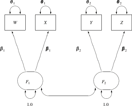
The hypothesis  requires that variables or tests under each factor are "interchangeable." In terms of the measurement model, several pairs
of parameters must be constrained to have equal estimates. That is, under the parallel-test model
requires that variables or tests under each factor are "interchangeable." In terms of the measurement model, several pairs
of parameters must be constrained to have equal estimates. That is, under the parallel-test model W and X should have the same effect or path coefficient  from their common factor
 F1, and they should also have the same measurement error variance  . Similarly,
 Y and Z should have the same effect or path coefficient  from their common factor
 F2, and they should also have the same measurement error variance  . These constraints are labeled in Figure 17.26.
You can impose each of these equality constraints by giving the same name for the parameters involved in the PATH model specification. The following statements specify the path diagram in Figure 17.26:
proc calis data=lord;
   path
      W <=== F1   = beta1,
      X <=== F1   = beta1,
      Y <=== F2   = beta2,
      Z <=== F2   = beta2;
   pvar
      F1  = 1.0,
      F2  = 1.0,
      W X = 2 * theta1,
      Y Z = 2 * theta2;
   pcov
      F1 F2;
run;
Note that the specification 2*theta1 in the PVAR statement means that theta1 is specified twice for the error variances of the two variables W and X. Similarly for the specification 2*theta2. An annotated fit summary is displayed in Figure 17.27.
Figure 17.27: Fit Summary, H2: Two-Factor Model with Parallel Tests for Lord Data
The chi-square value is 1.9335 (df=5, p=0.8583). This indicates that you cannot reject the hypothesized model H2. The standardized root mean square error (SRMSR) is 0.0076, which indicates a very good fit. Bentler’s comparative fit index is 1.0000. The adjusted GFI (AGFI) is 0.9970, and the RMSEA is close to zero. All results indicate that this is a good model for the data.
The estimation results are displayed in Figure 17.28.
Figure 17.28: Estimation Results, H2: Two-Factor Model with Parallel Tests for Lord Data
Notice that because you explicitly specify the parameter names for the path coefficients (that is, beta1 and beta2), they are used in the output shown in Figure 17.28. The correlation between F1 and F2 is 0.8987, which is a very high correlation that suggests F1 and F2 might have been the same factor in the population. The next section sets this value to one so that the current model becomes
a one-factor model with parallel tests.