The POWER Procedure
- Overview
-
Getting Started

-
Syntax
-
Details
-
ExamplesOne-Way ANOVAThe Sawtooth Power Function in Proportion AnalysesSimple AB/BA Crossover DesignsNoninferiority Test with Lognormal DataMultiple Regression and CorrelationComparing Two Survival CurvesConfidence Interval PrecisionCustomizing PlotsBinary Logistic Regression with Independent PredictorsWilcoxon-Mann-Whitney Test
- References
The method is from Lakatos (1988) and Cantor (1997, pp. 83–92).
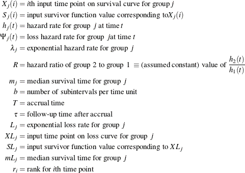
Define the following notation:
Each survival curve can be specified in one of several ways.
-
For exponential curves:
-
a single point
 on the curve
-
median survival time
-
hazard rate
-
hazard ratio (for curve 2, with respect to curve 1)
-
-
For piecewise linear curves with proportional hazards:
-
a set of points
 (for curve 1)
-
hazard ratio (for curve 2, with respect to curve 1)
-
-
For arbitrary piecewise linear curves:
-
a set of points

-
A total of ![]() evenly spaced time points
evenly spaced time points ![]() are used in calculations, where
are used in calculations, where
The hazard function is calculated for each survival curve at each time point. For an exponential curve, the (constant) hazard is given by one of the following, depending on the input parameterization:
![\[ h_ j(t) = \left\{ \begin{array}{l} \lambda _ j \\ \lambda _1 R \\ \frac{-\log (\frac{1}{2})}{m_ j} \\ \frac{-\log (S_ j(1))}{X_ j(1)} \\ \frac{-\log (S_1(1))}{X_1(1)} R \\ \end{array} \right. \]](images/statug_power0477.png)
For a piecewise linear curve, define the following additional notation:
The hazard is computed by using linear interpolation as follows:
With proportional hazards, the hazard rate of group 2’s curve in terms of the hazard rate of group 1’s curve is
Hazard function values ![]() for the loss curves are computed in an analogous way from
for the loss curves are computed in an analogous way from ![]() .
.
The expected number at risk ![]() at time i in group j is calculated for each group and time points 0 through M – 1, as follows:
at time i in group j is calculated for each group and time points 0 through M – 1, as follows:
![\begin{align*} N_ j(0) & = N w_ j \\ N_ j(i+1) & = N_ j(i) \left[ 1 - h_ j(t_ i) \left( \frac{1}{b} \right) - \Psi _ j (t_ i) \left( \frac{1}{b} \right) - \left( \frac{1}{b(T + \tau - t_ i)} \right) 1_{\{ t_ i > \tau \} } \right] \\ \end{align*}](images/statug_power0484.png)
Define ![]() as the ratio of hazards and
as the ratio of hazards and ![]() as the ratio of expected numbers at risk for time
as the ratio of expected numbers at risk for time ![]() :
:

The expected number of deaths in each subinterval is calculated as follows:
The rank values are calculated as follows according to which test statistic is used:
![\[ r_ i = \left\{ \begin{array}{ll} 1, & \mbox{log-rank} \\ N_1(i) + N_2(i), & \mbox{Gehan} \\ \sqrt {N_1(i) + N_2(i)}, & \mbox{Tarone-Ware} \\ \end{array} \right. \]](images/statug_power0490.png)
The distribution of the test statistic is approximated by ![]() where
where
![\[ E = \frac{\sum _{i=0}^{M-1} D_ i r_ i \left[ \frac{\phi _ i \theta _ i}{1 + \phi _ i \theta _ i} - \frac{\phi _ i}{1 + \phi _ i} \right] }{\sqrt {\sum _{i=0}^{M-1} D_ i r_ i^2 \frac{\phi _ i}{(1 + \phi _ i)^2} } } \]](images/statug_power0492.png)
Note that ![]() can be factored out of the mean E, and so it can be expressed equivalently as
can be factored out of the mean E, and so it can be expressed equivalently as
![\[ E = N^\frac {1}{2} E^\star = N^\frac {1}{2} \left[ \frac{\sum _{i=0}^{M-1} D_ i^\star r_ i^\star \left[ \frac{\phi _ i \theta _ i}{1 + \phi _ i \theta _ i} - \frac{\phi _ i}{1 + \phi _ i} \right] }{\sqrt {\sum _{i=0}^{M-1} D_ i^\star {r_ i^\star }^2 \frac{\phi _ i}{(1 + \phi _ i)^2} } } \right] \]](images/statug_power0494.png)
where ![]() is free of N and
is free of N and
![\begin{align*} D_ i^\star & = \left[ h_1(t_ i) N_1^\star (i) + h_2(t_ i) N_2^\star (i) \right] \left( \frac{1}{b} \right) \\ r_ i^\star & = \left\{ \begin{array}{ll} 1, & \mbox{log-rank} \\ N_1^\star (i) + N_2^\star (i), & \mbox{Gehan} \\ \sqrt {N_1^\star (i) + N_2^\star (i)}, & \mbox{Tarone-Ware} \\ \end{array} \right. \\ N_ j^\star (0) & = w_ j \\ N_ j^\star (i+1) & = N_ j^\star (i) \left[ 1 - h_ j(t_ i) \left( \frac{1}{b} \right) - \Psi _ j (t_ i) \left( \frac{1}{b} \right) - \left( \frac{1}{b(T + \tau - t_ i)} \right) 1_{\{ t_ i > \tau \} } \right] \\ \end{align*}](images/statug_power0496.png)
The approximate power is
![\[ \mr{power} = \left\{ \begin{array}{ll} \Phi \left( - N^\frac {1}{2} E^\star - z_{1-\alpha } \right), & \mbox{upper one-sided} \\ \Phi \left( N^\frac {1}{2} E^\star - z_{1-\alpha } \right), & \mbox{lower one-sided} \\ \Phi \left( - N^\frac {1}{2} E^\star - z_{1-\frac{\alpha }{2}} \right) + \Phi \left( N^\frac {1}{2} E^\star - z_{1-\frac{\alpha }{2}} \right), & \mbox{two-sided} \\ \end{array} \right. \\ \]](images/statug_power0497.png)
Note that the upper and lower one-sided cases are expressed differently than in other analyses. This is because ![]() corresponds to a higher survival curve in group 1 and thus, by the convention used in PROC power for two-group analyses,
the lower side.
corresponds to a higher survival curve in group 1 and thus, by the convention used in PROC power for two-group analyses,
the lower side.
For the one-sided cases, a closed-form inversion of the power equation yield an approximate total sample size
For the two-sided case, the solution for N is obtained by numerically inverting the power equation.
Accrual rates are converted to and from sample sizes according to the equation ![]() , where
, where ![]() is the accrual rate for group j.
is the accrual rate for group j.
Expected numbers of events—that is, deaths, whether observed or censored—are converted to and from sample sizes according to the equation
where ![]() is the expected number of events in group j. For an exponential curve, the equation simplifies to
is the expected number of events in group j. For an exponential curve, the equation simplifies to
For a piecewise linear curve, first define ![]() as the number of time points in the following collection:
as the number of time points in the following collection: ![]() ,
, ![]() , and input time points for group j strictly between
, and input time points for group j strictly between ![]() and
and ![]() . Denote the ordered set of these points as
. Denote the ordered set of these points as ![]() . The survival function values
. The survival function values ![]() and
and ![]() are calculated by linear interpolation between adjacent input time points if they do not coincide with any input time points.
Then the equation for a piecewise linear curve simplifies to
are calculated by linear interpolation between adjacent input time points if they do not coincide with any input time points.
Then the equation for a piecewise linear curve simplifies to