The POWER Procedure
- Overview
-
Getting Started

-
Syntax
-
Details
-
ExamplesOne-Way ANOVAThe Sawtooth Power Function in Proportion AnalysesSimple AB/BA Crossover DesignsNoninferiority Test with Lognormal DataMultiple Regression and CorrelationComparing Two Survival CurvesConfidence Interval PrecisionCustomizing PlotsBinary Logistic Regression with Independent PredictorsWilcoxon-Mann-Whitney Test
- References
Fisher’s z transformation (Fisher, 1921) of the sample correlation ![]() is defined as
is defined as
Fisher’s z test assumes the approximate normal distribution ![]() for z, where
for z, where
and
where ![]() is the number of variables partialed out (Anderson, 1984, pp. 132–133) and
is the number of variables partialed out (Anderson, 1984, pp. 132–133) and ![]() is the partial correlation between Y and
is the partial correlation between Y and ![]() adjusting for the set of zero or more variables
adjusting for the set of zero or more variables ![]() .
.
The test statistic
is assumed to have a normal distribution ![]() , where
, where ![]() is the null partial correlation and
is the null partial correlation and ![]() and
and ![]() are derived from Section 16.33 of Stuart and Ord (1994):
are derived from Section 16.33 of Stuart and Ord (1994):
![\begin{align*} \delta & = (N-3-p^\star )^{\frac{1}{2}} \left[ \frac{1}{2} \log \left( \frac{1+\rho _{Y|(X_1,X_{-1})}}{1-\rho _{Y|(X_1,X_{-1})}} \right) + \frac{\rho _{Y|(X_1,X_{-1})}}{2(N - 1 - p^\star )} \left( 1 + \frac{5 + \rho ^2_{Y|(X_1,X_{-1})}}{4(N - 1 - p^\star )} + \right. \right. \\ & \quad \left. \left. \frac{11 + 2 \rho ^2_{Y|(X_1,X_{-1})} + 3 \rho ^4_{Y|(X_1,X_{-1})}}{8(N - 1 - p^\star )^2} \right) - \frac{1}{2} \log \left( \frac{1+\rho _0}{1-\rho _0} \right) - \frac{\rho _0}{2(N - 1 - p^\star )} \right] \\ \nu & = \frac{N-3-p^\star }{N-1-p^\star } \left[ 1 + \frac{4 - \rho ^2_{Y|(X_1,X_{-1})}}{2(N - 1 - p^\star )} + \frac{22 - 6 \rho ^2_{Y|(X_1,X_{-1})} - 3 \rho ^4_{Y|(X_1,X_{-1})}}{6(N - 1 - p^\star )^2} \right] \\ \end{align*}](images/statug_power0133.png)
The approximate power is computed as
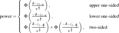
Because the test is biased, the achieved significance level might differ from the nominal significance level. The actual
alpha is computed in the same way as the power, except that the correlation ![]() is replaced by the null correlation
is replaced by the null correlation ![]() .
.
The two-sided case is identical to multiple regression with an intercept and ![]() , which is discussed in the section Analyses in the MULTREG Statement.
, which is discussed in the section Analyses in the MULTREG Statement.
Let ![]() denote the number of variables partialed out. For the one-sided cases, the test statistic is
denote the number of variables partialed out. For the one-sided cases, the test statistic is
![\[ t = (N-2-p^\star )^\frac {1}{2} \frac{R_{Y X_1|X_{-1}}}{\left(1 - R^2_{Y X_1|X_{-1}}\right)^\frac {1}{2}} \]](images/statug_power0136.png)
which is assumed to have a null distribution of ![]() .
.
If the X and Y variables are assumed to have a joint multivariate normal distribution, then the exact power is given by the following formula:
![\begin{align*} \mr{power} & = \left\{ \begin{array}{ll} P\left[ (N-2-p^\star )^\frac {1}{2} \frac{R_{Y X_1|X_{-1}}}{\left(1 - R^2_{Y X_1|X_{-1}}\right)^\frac {1}{2}} \ge t_{1-\alpha }(N-2-p^\star )\right], & \mbox{upper one-sided} \\ P\left[ (N-2-p^\star )^\frac {1}{2} \frac{R_{Y X_1|X_{-1}}}{\left(1 - R^2_{Y X_1|X_{-1}}\right)^\frac {1}{2}} \le t_{\alpha }(N-2-p^\star )\right], & \mbox{lower one-sided} \\ \end{array} \right. \\ & = \left\{ \begin{array}{ll} P\left[ R_{Y|(X_1,X_{-1})} \ge \frac{t_{1-\alpha }(N-2-p^\star )}{\left(t^2_{1-\alpha }(N-2-p^\star ) + N-2-p^\star \right)^\frac {1}{2}} \right], & \mbox{upper one-sided} \\ P\left[ R_{Y|(X_1,X_{-1})} \le \frac{t_{\alpha }(N-2-p^\star )}{\left(t^2_{\alpha }(N-2-p^\star ) + N-2-p^\star \right)^\frac {1}{2}} \right], & \mbox{lower one-sided} \\ \end{array} \right. \\ \end{align*}](images/statug_power0138.png)
The distribution of ![]() (given the underlying true correlation
(given the underlying true correlation ![]() ) is given in Chapter 32 of Johnson, Kotz, and Balakrishnan (1995).
) is given in Chapter 32 of Johnson, Kotz, and Balakrishnan (1995).
If the X variables are assumed to have fixed values, then the exact power is given by the noncentral t distribution ![]() , where the noncentrality is
, where the noncentrality is
![\[ \delta = N^\frac {1}{2} \frac{\rho _{Y X_1|X_{-1}}}{\left(1 - \rho ^2_{Y X_1|X_{-1}}\right)^\frac {1}{2}} \]](images/statug_power0140.png)
The power is