The Four Types of Estimable Functions
For main-effects models and regression models, the general form of estimable functions can be manipulated to provide tests of hypotheses involving only the parameters of the effect in question. The same result can also be obtained by entering each effect in turn as the last effect in the model and obtaining the Type I SS for that effect. These are the Type II SS. Using a modified reversible sweep operator, it is possible to obtain the Type II SS without actually refitting the model.
Thus, the Type II SS correspond to the R notation in which each effect is adjusted for all other appropriate effects. For a regression model such as
the Type II SS correspond to
|
Effect |
Type II SS |
|
|---|---|---|
|
|
|
|
|
|
|
|
|
|
|
For a main-effects model (A, B, and C as classification variables), the Type II SS correspond to
|
Effect |
Type II SS |
|
|---|---|---|
|
A |
|
|
|
B |
|
|
|
C |
|
As the discussion in the section A Three-Factor Main-Effects Model indicates, for regression and main-effects models the Type II SS provide an MRH for each effect that does not involve the parameters of the other effects.
In order to see what effects are appropriate to adjust for in computing Type II estimable functions, note that for models involving interactions and nested effects, in the absence of a priori parametric restrictions, it is not possible to obtain a test of a hypothesis for a main effect free of parameters of higher-level interactions effects with which the main effect is involved. It is reasonable to assume, then, that any test of a hypothesis concerning an effect should involve the parameters of that effect and only those other parameters with which that effect is involved. The concept of effect containment helps to define this involvement.
Given two effects F1 and F2, F1 is said to be contained in F2 provided that the following two conditions are met:
-
Both effects involve the same continuous variables (if any).
-
F2 has more CLASS variables than F1 does, and if F1 has CLASS variables, they all appear in F2.
Note that the intercept effect ![]() is contained in all pure CLASS effects, but it is not contained in any effect involving a continuous variable. No effect
is contained by
is contained in all pure CLASS effects, but it is not contained in any effect involving a continuous variable. No effect
is contained by ![]() .
.
Type II, Type III, and Type IV estimable functions rely on this definition, and they all have one thing in common: the estimable functions involving an effect F1 also involve the parameters of all effects that contain F1, and they do not involve the parameters of effects that do not contain F1 (other than F1).
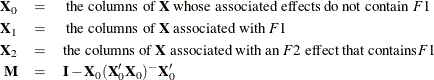
The Type II estimable functions for an effect F1 have an ![]() (before reduction to full row rank) of the following form:
(before reduction to full row rank) of the following form:
-
All columns of
 associated with effects not containing F1 (except F1) are zero.
-
The submatrix of
associated with effect F1 is 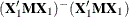 .
.
-
Each of the remaining submatrices of
associated with an effect F2 that contains F1 is 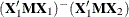 .
.
In these submatrices,
For the model
class A B;
model Y = A B A*B;
the Type II SS correspond to
for effects A, B, and A * B, respectively. For the model
class A B C;
model Y =  A B(A) C(A B);
the Type II SS correspond to
for effects A, ![]() and
and ![]() , respectively. For the model
, respectively. For the model
model Y = x x*x;
the Type II SS correspond to
for x and ![]() , respectively.
, respectively.
Note that, as in the situation for Type I tests, PROC MIXED and PROC GLIMMIX compute Type I hypotheses by sweeping ![]() , but their test statistics are not necessarily equivalent to the results of sequentially fitting with those procedures models
that contain successively more effects; while PROC TRANSREG computes tests labeled as being Type II by leaving out each effect
in turn, but the specific linear hypotheses associated with these tests might not be precisely the same as the ones derived
from successively sweeping
, but their test statistics are not necessarily equivalent to the results of sequentially fitting with those procedures models
that contain successively more effects; while PROC TRANSREG computes tests labeled as being Type II by leaving out each effect
in turn, but the specific linear hypotheses associated with these tests might not be precisely the same as the ones derived
from successively sweeping ![]() .
.
For a ![]() factorial with w observations per cell, the general form of estimable functions is shown in Table 15.5. Any nonzero values for L2, L4, and L6 can be used to construct
factorial with w observations per cell, the general form of estimable functions is shown in Table 15.5. Any nonzero values for L2, L4, and L6 can be used to construct ![]() vectors for computing the Type II SS for A, B, and A * B, respectively.
vectors for computing the Type II SS for A, B, and A * B, respectively.
Table 15.5: General Form of Estimable Functions for ![]() Factorial
Factorial
|
Effect |
Coefficient |
|
|---|---|---|
|
|
L1 |
|
|
A1 |
L2 |
|
|
A2 |
L1 – L2 |
|
|
B1 |
L4 |
|
|
B2 |
L1 – L4 |
|
|
AB11 |
L6 |
|
|
AB12 |
L2 – L6 |
|
|
AB21 |
L4 – L6 |
|
|
AB22 |
L1 – L2 – L4 + L6 |
For a balanced ![]() factorial with the same number of observations in every cell, the Type II estimable functions are shown in Table 15.6.
factorial with the same number of observations in every cell, the Type II estimable functions are shown in Table 15.6.
Table 15.6: Type II Estimable Functions for Balanced ![]() Factorial
Factorial
|
Coefficients for Effect |
||||||
|---|---|---|---|---|---|---|
|
Effect |
A |
B |
A * B |
|||
|
|
0 |
0 |
0 |
|||
|
A1 |
L2 |
0 |
0 |
|||
|
A2 |
–L2 |
0 |
0 |
|||
|
B1 |
0 |
L4 |
0 |
|||
|
B2 |
0 |
–L4 |
0 |
|||
|
AB11 |
0.5 |
0.5 |
L6 |
|||
|
AB12 |
0.5 |
–0.5 |
–L6 |
|||
|
AB21 |
–0.5 |
0.5 |
–L6 |
|||
|
AB22 |
–0.5 |
–0.5 |
L6 |
|||
Now consider an unbalanced ![]() factorial with two observations in every cell except the AB22 cell, which contains only one observation. The general form of estimable functions is the same as if it were balanced, since
the same effects are still estimable. However, the Type II estimable functions for A and B are not the same as they were for the balanced design. The Type II estimable functions for this unbalanced
factorial with two observations in every cell except the AB22 cell, which contains only one observation. The general form of estimable functions is the same as if it were balanced, since
the same effects are still estimable. However, the Type II estimable functions for A and B are not the same as they were for the balanced design. The Type II estimable functions for this unbalanced ![]() factorial are shown in Table 15.7.
factorial are shown in Table 15.7.
Table 15.7: Type II Estimable Functions for Unbalanced ![]() Factorial
Factorial
|
Coefficients for Effect |
||||||
|---|---|---|---|---|---|---|
|
Effect |
A |
B |
A * B |
|||
|
|
0 |
0 |
0 |
|||
|
A1 |
L2 |
0 |
0 |
|||
|
A2 |
–L2 |
0 |
0 |
|||
|
B1 |
0 |
L4 |
0 |
|||
|
B2 |
0 |
–L4 |
0 |
|||
|
AB11 |
0.6 |
0.6 |
L6 |
|||
|
AB12 |
0.4 |
–0.6 |
–L6 |
|||
|
AB21 |
–0.6 |
0.4 |
–L6 |
|||
|
AB22 |
–0.4 |
–0.4 |
L6 |
|||
By comparing the hypothesis being tested in the balanced case to the hypothesis being tested in the unbalanced case for effects A and B, you can note that the Type II hypotheses for A and B are dependent on the cell frequencies in the design. For unbalanced designs in which the cell frequencies are not proportional to the background population, the Type II hypotheses for effects that are contained in other effects are of questionable value.
However, if an effect is not contained in any other effect, the Type II hypothesis for that effect is an MRH that does not involve any parameters except those associated with the effect in question.
Thus, Type II SS are appropriate for the following models:
-
any balanced model
-
any main-effects model
-
any pure regression model
-
an effect not contained in any other effect (regardless of the model)
In addition to the preceding models, Type II SS are generally accepted by most statisticians for purely nested models.