Introduction to Discriminant Procedures
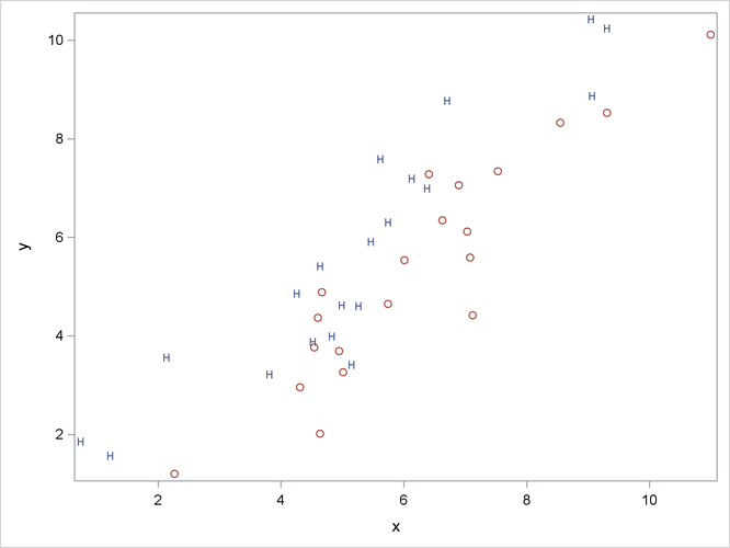
Consider an artificial data set with two classes of observations indicated by 'H' and 'O'. The following statements generate and plot the data:
data random;
   drop n;

   Group = 'H';
   do n = 1 to 20;
      x = 4.5 + 2 * normal(57391);
      y = x + .5 + normal(57391);
      output;
   end;

   Group = 'O';
   do n = 1 to 20;
      x = 6.25 + 2 * normal(57391);
      y = x - 1 + normal(57391);
      output;
   end;

run;

proc sgplot noautolegend;
   scatter y=y x=x / markerchar=group group=group;
run;
The plot is shown in Figure 10.1.
The following statements perform a canonical discriminant analysis and display the results in Figure 10.2:
proc candisc anova;
   class Group;
   var x y;
run;
Figure 10.2: Contrasting Univariate and Multivariate Analyses
| Univariate Test Statistics | |||||||
|---|---|---|---|---|---|---|---|
| F Statistics, Num DF=1, Den DF=38 | |||||||
| Variable | Total Standard Deviation |
Pooled Standard Deviation |
Between Standard Deviation |
R-Square | R-Square / (1-RSq) |
F Value | Pr > F |
| x | 2.1776 | 2.1498 | 0.6820 | 0.0503 | 0.0530 | 2.01 | 0.1641 |
| y | 2.4215 | 2.4486 | 0.2047 | 0.0037 | 0.0037 | 0.14 | 0.7105 |
| Canonical Correlation |
Adjusted Canonical Correlation |
Approximate Standard Error |
Squared Canonical Correlation |
Eigenvalues of Inv(E)*H = CanRsq/(1-CanRsq) |
Test of H0: The canonical correlations in the current row and all that follow are zero | ||||||||
|---|---|---|---|---|---|---|---|---|---|---|---|---|---|
| Eigenvalue | Difference | Proportion | Cumulative | Likelihood Ratio |
Approximate F Value |
Num DF | Den DF | Pr > F | |||||
| 1 | 0.598300 | 0.589467 | 0.102808 | 0.357963 | 0.5575 | 1.0000 | 1.0000 | 0.64203704 | 10.31 | 2 | 37 | 0.0003 | |
| Note: | The F statistic is exact. |
The univariate R squares are very small, 0.0503 for x and 0.0037 for y, and neither variable shows a significant difference between the classes at the 0.10 level.
The multivariate test for differences between the classes is significant at the 0.0003 level. Thus, the multivariate analysis
has found a highly significant difference, whereas the univariate analyses failed to achieve even the 0.10 level. The raw
canonical coefficients for the first canonical variable, Can1, show that the classes differ most widely on the linear combination -1.205756217 x + 1.010412967 y or approximately y - 1.2 x. The R square between Can1 and the CLASS variable is 0.357963 as given by the squared canonical correlation, which is much higher than either univariate
R square.
In this example, the variables are highly correlated within classes. If the within-class correlation were smaller, there would be greater agreement between the univariate and multivariate analyses.