Introduction to Structural Equation Modeling with Latent Variables
The model analyzed by Jöreskog and Sörbom (1988) is displayed in the path diagram in Figure 17.39.
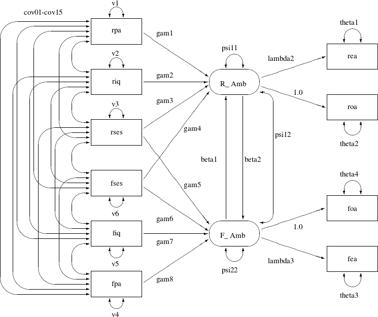
Two latent variables, R_Amb and F_Amb, represent the respondent’s level of ambition and his best friend’s level of ambition, respectively. The model states that
the respondent’s ambition (R_Amb) is determined by his intelligence (riq) and socioeconomic status (rses), his perception of his parents’ aspiration for him (rpa), and his friend’s socioeconomic status (fses) and ambition (F_Amb). It is assumed that his friend’s intelligence (fiq) and parental aspiration (fpa) affect the respondent’s ambition only indirectly through the friend’s ambition (F_Amb). Ambition is indicated by the manifest variables of occupational (roa) and educational aspiration (rea), which are assumed to have uncorrelated residuals. The path coefficient from ambition to occupational aspiration is set
to 1.0 to determine the scale of the ambition latent variable.
The path diagram shown in Figure 17.39 appears to be very complicated. Sometimes when researchers draw their path diagram with a lot of variables, they omit the
covariances among exogenous variables for overall clarity. For example, the double-headed paths that represent cov01–cov15 in Figure 17.39 can be omitted. In addition, unconstrained variance and error variance parameters in the path diagram could be omitted without
losing the pertinent information in the path diagram. For example, variance parameters v1–v6 and error variance parameters theta1–theta4 in Figure 17.39 detract from the main focus on the functional relationships of the model.
These omissions in the path diagram are in fact inconsequential when you transcribe them into the PATH model in PROC CALIS. The reason is that PROC CALIS employs several useful default parameterization rules that make the model specification process much easier and more intuitive. Here are the sets of default covariance structure parameters in the PATH modeling language:
-
variances for all exogenous (observed or latent) variables
-
error variances of all endogenous (observed or latent) variables
-
covariances among all exogenous (observed or latent, excluding error) variables
For example, these rules for setting default covariance structure parameters mean that the following sets of parameters in Figure 17.39 are optional in the path diagram representation and in the corresponding PATH model specification:
-
v1–v6 -
theta1–theta4,psi11, andpsi22 -
cov01–cov15
Note that the double-headed path labeled with psi12, which is a covariance parameter among error terms for R_Amb and F_Amb, is not a default parameter. As a result, it must be represented in the path diagram and in the PATH model specification.
Another simplification is to omit the unconstrained parameter names in the path diagram. In the PATH model specification, an "unnamed" parameter is a free parameter by default—there is no need to give unique names to denote free parameters. With all the mentioned simplifications, you can depict your path diagram simply as the one in Figure 17.40.
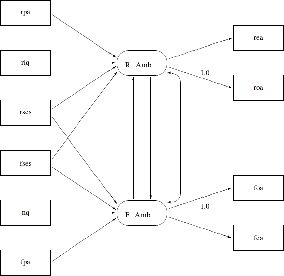
The simplified path diagram in Figure 17.40 is readily transcribed into the PATH model as shown in the following statements:
proc calis data=aspire nobs=329;
   path
      /* structural model of influences */
      R_Amb <=== rpa     ,
      R_Amb <=== riq     ,
      R_Amb <=== rses    ,
      R_Amb <=== fses    ,
      F_Amb <=== rses    ,
      F_Amb <=== fses    ,
      F_Amb <=== fiq     ,
      F_Amb <=== fpa     ,
      R_Amb <=== F_Amb   ,
      F_Amb <=== R_Amb   ,

      /* measurement model for aspiration */
      rea <===  R_Amb      ,
      roa <===  R_Amb  = 1.,
      foa <===  F_Amb  = 1.,
      fea <===  F_Amb    ;
   pcov
      R_Amb  F_Amb;
run;
Again, because you have 15 paths (single- or double- headed) in the path diagram, you expect that there are 15 entries in
the PATH and the PCOV statements. Essentially, in this PATH model specification you specify all the functional relationships
(single-headed arrows) in the path diagram and the covariance of error terms (double-headed arrows) for R_Amb and F_Amb.
Since this TYPE=CORR data set does not contain an observation with _TYPE_=N giving the sample size, it is necessary to specify the NOBS= option in the PROC CALIS statement.
The fit summary is displayed in Figure 17.41, and the estimation results are displayed in Figure 17.42.
The model fit chi-square value is 26.6972 (df=15, p=0.0313). From the hypothesis testing point of view, this result says that this is an extreme sample given the model is true; therefore, the model should be rejected. But in social and behavioral sciences, you rarely abandon a model purely on the ground of chi-square significance test. The main reason is that you might only need to find a model that is approximately true, but the hypothesis testing framework is for testing exact model representation in the population. To determine whether a model is good or bad, you usually consult other fit indices. Several fit indices are shown in Figure 17.41.
The standardized RMSR is 0.0202. The RMSEA value is 0.0488. Both of these indices are smaller than 0.05, which indicate good model fit by convention. The adjusted GFI is 0.9428, and the comparative fit index is 0.9859. Again, values greater than 0.9 for these indices indicate good model fit by convention. Therefore, you can conclude that this is a good model for the data. Akaike’s information criterion (AIC) and the Schwarz Bayesian criterion are also shown. You cannot interpret these values directly, but they are useful for model comparison given the same data, as shown in later sections.
Figure 17.42: Career Aspiration Data: Estimation Results for Analysis 1
| PATH List | |||||||
|---|---|---|---|---|---|---|---|
| Path | Parameter | Estimate | Standard Error |
t Value | Pr > |t| | ||
| R_Amb | <=== | rpa | _Parm01 | 0.16122 | 0.03879 | 4.1560 | <.0001 |
| R_Amb | <=== | riq | _Parm02 | 0.24965 | 0.04398 | 5.6763 | <.0001 |
| R_Amb | <=== | rses | _Parm03 | 0.21840 | 0.04420 | 4.9415 | <.0001 |
| R_Amb | <=== | fses | _Parm04 | 0.07184 | 0.04971 | 1.4453 | 0.1484 |
| F_Amb | <=== | rses | _Parm05 | 0.05754 | 0.04812 | 1.1956 | 0.2318 |
| F_Amb | <=== | fses | _Parm06 | 0.21278 | 0.04169 | 5.1042 | <.0001 |
| F_Amb | <=== | fiq | _Parm07 | 0.32451 | 0.04352 | 7.4562 | <.0001 |
| F_Amb | <=== | fpa | _Parm08 | 0.14832 | 0.03645 | 4.0696 | <.0001 |
| R_Amb | <=== | F_Amb | _Parm09 | 0.19816 | 0.10228 | 1.9374 | 0.0527 |
| F_Amb | <=== | R_Amb | _Parm10 | 0.21893 | 0.11125 | 1.9680 | 0.0491 |
| rea | <=== | R_Amb | _Parm11 | 1.06268 | 0.09014 | 11.7894 | <.0001 |
| roa | <=== | R_Amb | 1.00000 | ||||
| foa | <=== | F_Amb | 1.00000 | ||||
| fea | <=== | F_Amb | _Parm12 | 1.07558 | 0.08131 | 13.2287 | <.0001 |
| Variance Parameters | ||||||
|---|---|---|---|---|---|---|
| Variance Type |
Variable | Parameter | Estimate | Standard Error |
t Value | Pr > |t| |
| Exogenous | riq | _Add01 | 1.00000 | 0.07809 | 12.8062 | <.0001 |
| rpa | _Add02 | 1.00000 | 0.07809 | 12.8062 | <.0001 | |
| rses | _Add03 | 1.00000 | 0.07809 | 12.8062 | <.0001 | |
| fiq | _Add04 | 1.00000 | 0.07809 | 12.8062 | <.0001 | |
| fpa | _Add05 | 1.00000 | 0.07809 | 12.8062 | <.0001 | |
| fses | _Add06 | 1.00000 | 0.07809 | 12.8062 | <.0001 | |
| Error | roa | _Add07 | 0.41215 | 0.05122 | 8.0458 | <.0001 |
| rea | _Add08 | 0.33614 | 0.05210 | 6.4519 | <.0001 | |
| foa | _Add09 | 0.40460 | 0.04618 | 8.7606 | <.0001 | |
| fea | _Add10 | 0.31120 | 0.04593 | 6.7759 | <.0001 | |
| R_Amb | _Add11 | 0.28099 | 0.04623 | 6.0778 | <.0001 | |
| F_Amb | _Add12 | 0.22806 | 0.03850 | 5.9233 | <.0001 | |
| Covariances Among Exogenous Variables | ||||||
|---|---|---|---|---|---|---|
| Var1 | Var2 | Parameter | Estimate | Standard Error |
t Value | Pr > |t| |
| rpa | riq | _Add13 | 0.18390 | 0.05614 | 3.2756 | 0.0011 |
| rses | riq | _Add14 | 0.22200 | 0.05656 | 3.9250 | <.0001 |
| rses | rpa | _Add15 | 0.04890 | 0.05528 | 0.8846 | 0.3764 |
| fiq | riq | _Add16 | 0.33550 | 0.05824 | 5.7606 | <.0001 |
| fiq | rpa | _Add17 | 0.07820 | 0.05538 | 1.4120 | 0.1580 |
| fiq | rses | _Add18 | 0.23020 | 0.05666 | 4.0628 | <.0001 |
| fpa | riq | _Add19 | 0.10210 | 0.05550 | 1.8395 | 0.0658 |
| fpa | rpa | _Add20 | 0.11470 | 0.05558 | 2.0638 | 0.0390 |
| fpa | rses | _Add21 | 0.09310 | 0.05545 | 1.6789 | 0.0932 |
| fpa | fiq | _Add22 | 0.20870 | 0.05641 | 3.7000 | 0.0002 |
| fses | riq | _Add23 | 0.18610 | 0.05616 | 3.3135 | 0.0009 |
| fses | rpa | _Add24 | 0.01860 | 0.05523 | 0.3368 | 0.7363 |
| fses | rses | _Add25 | 0.27070 | 0.05720 | 4.7323 | <.0001 |
| fses | fiq | _Add26 | 0.29500 | 0.05757 | 5.1244 | <.0001 |
| fses | fpa | _Add27 | -0.04380 | 0.05527 | -0.7925 | 0.4281 |
In Figure 17.42, some of the paths do not show significance. That is, fses does not seem to be a good indicator of a respondent’s ambition R_Amb and rses does not seem to be a good indicator of a friend’s ambition F_Amb. The t values are 1.445 and 1.195, respectively, which are much smaller than the nominal 1.96 value at the 0.05 ![]() -level of significance. Other paths are either significant or marginally significant.
-level of significance. Other paths are either significant or marginally significant.
You should be very cautious about interpreting the current analysis results for two reasons. First, as mentioned previously the data consist of dependent observations, and it was not certain how the issue could have been addressed beyond setting the sample size to half of the actual size. Second, structural equation modeling methodology is mainly applicable when you analyze covariance structures. When you input a correlation matrix for analysis, there is no guarantee that the statistical tests and standard error estimates are applicable. You should view the interpretations made here just as an exercise of applying structural equation modeling.
In Figure 17.42, all parameter names are generated by PROC CALIS. Alternatively, you can also name these parameters in your PATH model specification. The following shows a PATH model specification that corresponds to the complete path diagram shown in Figure 17.39:
proc calis data=aspire nobs=329;
   path
      /* structural model of influences */
      rpa    ===>  R_Amb   =  gam1,
      riq    ===>  R_Amb   =  gam2,
      rses   ===>  R_Amb   =  gam3,
      fses   ===>  R_Amb   =  gam4,
      rses   ===>  F_Amb   =  gam5,
      fses   ===>  F_Amb   =  gam6,
      fiq    ===>  F_Amb   =  gam7,
      fpa    ===>  F_Amb   =  gam8,
      F_Amb  ===>  R_Amb   = beta1,
      R_Amb  ===>  F_Amb   = beta2,

      /* measurement model for aspiration */
      R_Amb  ===>  rea     = lambda2,
      R_Amb  ===>  roa     = 1.,
      F_Amb  ===>  foa     = 1.,
      F_Amb  ===>  fea     = lambda3;
   pvar
      R_Amb = psi11,
      F_Amb = psi22,
      rpa riq rses fpa fiq fses = v1-v6,
      rea roa fea foa = theta1-theta4;
   pcov
      R_Amb F_Amb = psi12,
      rpa riq rses fpa fiq fses = cov01-cov15;
run;
In this specification, the names of the parameters correspond to those used by Jöreskog and Sörbom (1988). Compared with the simplified version of the same model specification, you name 27 more parameters in the current specification. You have to be careful with this many parameters. If you inadvertently repeat the use of some parameter names, you will have unexpected constraints in the model.
The results from this analysis are displayed in Figure 17.43.
Figure 17.43: Career Aspiration Data: Estimation Results with Designated Parameter Names (Analysis 1)
| PATH List | |||||||
|---|---|---|---|---|---|---|---|
| Path | Parameter | Estimate | Standard Error |
t Value | Pr > |t| | ||
| rpa | ===> | R_Amb | gam1 | 0.16122 | 0.03879 | 4.1560 | <.0001 |
| riq | ===> | R_Amb | gam2 | 0.24965 | 0.04398 | 5.6763 | <.0001 |
| rses | ===> | R_Amb | gam3 | 0.21840 | 0.04420 | 4.9415 | <.0001 |
| fses | ===> | R_Amb | gam4 | 0.07184 | 0.04971 | 1.4453 | 0.1484 |
| rses | ===> | F_Amb | gam5 | 0.05754 | 0.04812 | 1.1956 | 0.2318 |
| fses | ===> | F_Amb | gam6 | 0.21278 | 0.04169 | 5.1042 | <.0001 |
| fiq | ===> | F_Amb | gam7 | 0.32451 | 0.04352 | 7.4562 | <.0001 |
| fpa | ===> | F_Amb | gam8 | 0.14832 | 0.03645 | 4.0696 | <.0001 |
| F_Amb | ===> | R_Amb | beta1 | 0.19816 | 0.10228 | 1.9374 | 0.0527 |
| R_Amb | ===> | F_Amb | beta2 | 0.21893 | 0.11125 | 1.9680 | 0.0491 |
| R_Amb | ===> | rea | lambda2 | 1.06268 | 0.09014 | 11.7894 | <.0001 |
| R_Amb | ===> | roa | 1.00000 | ||||
| F_Amb | ===> | foa | 1.00000 | ||||
| F_Amb | ===> | fea | lambda3 | 1.07558 | 0.08131 | 13.2287 | <.0001 |
| Variance Parameters | ||||||
|---|---|---|---|---|---|---|
| Variance Type |
Variable | Parameter | Estimate | Standard Error |
t Value | Pr > |t| |
| Error | R_Amb | psi11 | 0.28099 | 0.04623 | 6.0778 | <.0001 |
| F_Amb | psi22 | 0.22806 | 0.03850 | 5.9233 | <.0001 | |
| Exogenous | rpa | v1 | 1.00000 | 0.07809 | 12.8062 | <.0001 |
| riq | v2 | 1.00000 | 0.07809 | 12.8062 | <.0001 | |
| rses | v3 | 1.00000 | 0.07809 | 12.8062 | <.0001 | |
| fpa | v4 | 1.00000 | 0.07809 | 12.8062 | <.0001 | |
| fiq | v5 | 1.00000 | 0.07809 | 12.8062 | <.0001 | |
| fses | v6 | 1.00000 | 0.07809 | 12.8062 | <.0001 | |
| Error | rea | theta1 | 0.33614 | 0.05210 | 6.4519 | <.0001 |
| roa | theta2 | 0.41215 | 0.05122 | 8.0458 | <.0001 | |
| fea | theta3 | 0.31120 | 0.04593 | 6.7759 | <.0001 | |
| foa | theta4 | 0.40460 | 0.04618 | 8.7606 | <.0001 | |
| Covariances Among Exogenous Variables | ||||||
|---|---|---|---|---|---|---|
| Var1 | Var2 | Parameter | Estimate | Standard Error |
t Value | Pr > |t| |
| rpa | riq | cov01 | 0.18390 | 0.05614 | 3.2756 | 0.0011 |
| rpa | rses | cov02 | 0.04890 | 0.05528 | 0.8846 | 0.3764 |
| riq | rses | cov03 | 0.22200 | 0.05656 | 3.9250 | <.0001 |
| rpa | fpa | cov04 | 0.11470 | 0.05558 | 2.0638 | 0.0390 |
| riq | fpa | cov05 | 0.10210 | 0.05550 | 1.8395 | 0.0658 |
| rses | fpa | cov06 | 0.09310 | 0.05545 | 1.6789 | 0.0932 |
| rpa | fiq | cov07 | 0.07820 | 0.05538 | 1.4120 | 0.1580 |
| riq | fiq | cov08 | 0.33550 | 0.05824 | 5.7606 | <.0001 |
| rses | fiq | cov09 | 0.23020 | 0.05666 | 4.0628 | <.0001 |
| fpa | fiq | cov10 | 0.20870 | 0.05641 | 3.7000 | 0.0002 |
| rpa | fses | cov11 | 0.01860 | 0.05523 | 0.3368 | 0.7363 |
| riq | fses | cov12 | 0.18610 | 0.05616 | 3.3135 | 0.0009 |
| rses | fses | cov13 | 0.27070 | 0.05720 | 4.7323 | <.0001 |
| fpa | fses | cov14 | -0.04380 | 0.05527 | -0.7925 | 0.4281 |
| fiq | fses | cov15 | 0.29500 | 0.05757 | 5.1244 | <.0001 |
These are the same results as displayed in Figure 17.42 for the simplified PATH model specification. The only differences are the arrangement of estimation results and the naming of the parameters.