Introduction to Structural Equation Modeling with Latent Variables
In the preceding section, you use the FACTOR modeling language of PROC CALIS to specify the parallel tests model. This model has also been specified by the PATH modeling language in the section H2: Two-Factor Model with Parallel Tests for Lord Data. The two specifications are equivalent; they lead to the same model fitting and estimation results. The main reason for providing two different types of modeling languages in PROC CALIS is that different researchers come from different fields of applications. Some researchers might be more comfortable with the confirmatory factor tradition, and some might equate structural equation models with path diagrams for variables.
PROC CALIS has still another modeling language that is closely related to the path diagram representation: the RAM model specification. In this section, the parallel tests model (H2) described in H2: Two-Factor Model with Parallel Tests for Lord Data is used to illustrate the RAM model specification in PROC CALIS.
The path diagram for this model is reproduced in Figure 17.36.
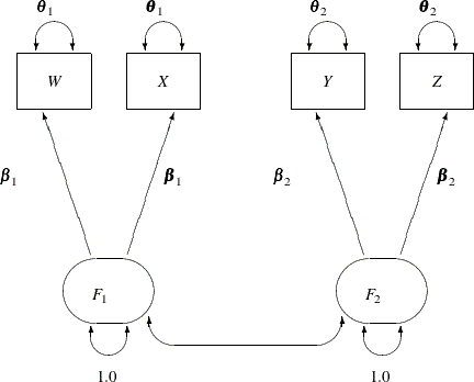
The path diagram in Figure 17.36 can be readily transcribed into the RAM model specification by following these simple rules:
-
Each single- or double- headed path corresponds to an entry in the RAM model specification.
-
The single-headed paths are specified with the _A_ path type or matrix keyword.
-
The double-headed paths are specified with the _P_ path type or matrix keyword.
At this point, you do not need to define the RAM model matrices _A_ and _P_, as long as you recognize that they are used as keywords to distinguish different path types. There are 11 single- or double- headed paths in Figure 17.36, and therefore you expect to specify these 11 elements in the RAM model, as shown in the following statements:
proc calis data=lord;
   ram var = W X Y Z F1 F2, /* W=1, X=2, Y=3, Z=4, F1=5, F2=6*/
       _A_   1  5  beta1,
       _A_   2  5  beta1,
       _A_   3  6  beta2,
       _A_   4  6  beta2,
       _P_   5  5  1.0,
       _P_   6  6  1.0,
       _P_   1  1  theta1,
       _P_   2  2  theta1,
       _P_   3  3  theta2,
       _P_   4  4  theta2,
       _P_   5  6  ;
run;
In this specification, the RAM statement invokes the RAM modeling language. The first option is the VAR= option where you
specify the variables, observed and latent, in the model. The order in the VAR= variable list represents the order of these
variables in the RAM model matrices. For this example, W is 1, X is 2, and so on. Next, you specify 11 RAM entries for the 11 path elements in the path diagram shown in Figure 17.36.
The first four entries are for the single-headed paths. They all begin with the _A_ keyword. In each of these _A_ entries, you specify the variable number of the outcome variable (being pointed at), and then the variable number of the
predictor variable. At the end of the entry, you can specify a parameter name, a fixed value, an initial value, or nothing.
In this example, all the _A_ entries are specified with parameter names. The first two paths are constrained because they use the same parameter name
beta1. The next two paths are constrained because they use the same parameter name beta2.
The rest of the RAM entries in the example are of the _P_ type, which is for the specification of variances or covariances in the RAM model (the double-headed arrows in the path diagram).
The _P_ entry with [5,5] is for the variance of the fifth variable, F1, on the VAR= list. This variance is fixed at 1.0 in the model, and so is the variance of the sixth variable, F2, in the next _P_ entry.
The next four _P_ entries are for the specification of error variances of the observed variables W, X, Y, and Z. You use the desired parameter names for constraining these parameters, as required in the parallel test model.
The last _P_ entry in the RAM statement is for the covariance between the fifth variable (F1) and the sixth variable (F2). You specify neither a parameter name nor a fixed value at the end of this entry. By default, this empty parameter specification
is treated as a free parameter in the model. A parameter name for this entry is generated by PROC CALIS.
The fit summary for this RAM model is shown in Figure 17.37, and the estimation results are shown in Figure 17.38.
Figure 17.38: Estimation Results of RAM Model with Parallel Tests for Lord Data
| RAM Pattern and Estimates | |||||||||
|---|---|---|---|---|---|---|---|---|---|
| Matrix | Row | Column | Parameter | Estimate | Standard Error |
t Value | Pr > |t| | ||
| _A_ (1) | W | 1 | F1 | 5 | beta1 | 7.60099 | 0.26844 | 28.3158 | <.0001 |
| X | 2 | F1 | 5 | beta1 | 7.60099 | 0.26844 | 28.3158 | <.0001 | |
| Y | 3 | F2 | 6 | beta2 | 8.59186 | 0.27967 | 30.7215 | <.0001 | |
| Z | 4 | F2 | 6 | beta2 | 8.59186 | 0.27967 | 30.7215 | <.0001 | |
| _P_ (2) | F1 | 5 | F1 | 5 | 1.00000 | ||||
| F2 | 6 | F2 | 6 | 1.00000 | |||||
| W | 1 | W | 1 | theta1 | 28.55545 | 1.58641 | 18.0000 | <.0001 | |
| X | 2 | X | 2 | theta1 | 28.55545 | 1.58641 | 18.0000 | <.0001 | |
| Y | 3 | Y | 3 | theta2 | 23.73200 | 1.31844 | 18.0000 | <.0001 | |
| Z | 4 | Z | 4 | theta2 | 23.73200 | 1.31844 | 18.0000 | <.0001 | |
| F1 | 5 | F2 | 6 | _Parm1 | 0.89864 | 0.01865 | 48.1801 | <.0001 | |
Again, the model fit and the estimation results match those from the PATH model specification in Figure 17.27 and Figure 17.28, and those from the FACTOR model specification in Figure 17.34 and Figure 17.35.