Introduction to Structural Equation Modeling with Latent Variables
Psychometric test theory involves many kinds of models that relate scores on psychological and educational tests to latent variables that represent intelligence or various underlying abilities. The following example uses data on four vocabulary tests from Lord (1957). Tests W and X have 15 items each and are administered with very liberal time limits. Tests Y and Z have 75 items and are administered under time pressure. The covariance matrix is read by the following DATA step:
data lord(type=cov);
   input _type_ $ _name_ $ W X Y Z;
   datalines;
n   . 649       .       .       .
cov W 86.3979   .       .       .
cov X 57.7751 86.2632   .       .
cov Y 56.8651 59.3177 97.2850   .
cov Z 58.8986 59.6683 73.8201 97.8192
;
The psychometric model of interest states that W and X are determined by a single common factor ![]() , and Y and Z are determined by a single common factor
, and Y and Z are determined by a single common factor ![]() . The two common factors are expected to have a positive correlation, and it is desired to estimate this correlation. It is
convenient to assume that the common factors have unit variance, so their correlation will be equal to their covariance. The
error terms for all the manifest variables are assumed to be uncorrelated with each other and with the common factors. The
model equations are
. The two common factors are expected to have a positive correlation, and it is desired to estimate this correlation. It is
convenient to assume that the common factors have unit variance, so their correlation will be equal to their covariance. The
error terms for all the manifest variables are assumed to be uncorrelated with each other and with the common factors. The
model equations are
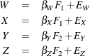
with the following assumptions:
The corresponding path diagram is shown in Figure 17.19.
In Figure 17.19, error terms are not explicitly represented, but error variances for the observed variables are represented by double-headed
arrows that point to the variables. The error variance parameters in the model are labeled with ![]() ,
, ![]() ,
, ![]() , and
, and ![]() , respectively, for the four observed variables. In the terminology of confirmatory factor analysis, these four variables
are called indicators of the corresponding latent factors
, respectively, for the four observed variables. In the terminology of confirmatory factor analysis, these four variables
are called indicators of the corresponding latent factors ![]() and
and ![]() .
.
Figure 17.19 represents the model equations clearly. It includes all the variables and the parameters in the diagram. However, sometimes researchers represent the same model with a simplified path diagram in which unconstrained parameters are not labeled, as shown in Figure 17.20.
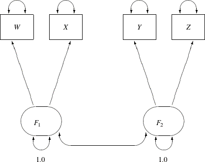
This simplified representation is also compatible with the PATH modeling language of PROC CALIS. In fact, this might be an easier starting point for modelers. With the following rules, the conversion from the path diagram to the PATH model specification is very straightforward:
-
Each single-headed arrow in the path diagram is specified in the PATH statement.
-
Each double-headed arrow that points to a single variable is specified in the PVAR statement.
-
Each double-headed arrow that points to two distinct variables is specified in the PCOV statement.
Hence, you can convert the simplified path diagram in Figure 17.20 easily to the following PATH model specification:
proc calis data=lord;
   path
      W <=== F1,
      X <=== F1,
      Y <=== F2,
      Z <=== F2;
   pvar
      F1 = 1.0,
      F2 = 1.0,
      W X Y Z;
   pcov
      F1 F2;
run;
In this specification, you do not need to specify the parameter names. However, you do need to specify fixed values specified
in the path diagram. For example, the variances of F1 and F2 are both fixed at 1 in the PVAR statement.
These fixed variances are applied solely for the purpose of model identification. Because F1 and F2 are latent variables and their scales are arbitrary, fixing their scales are necessary for model identification. Beyond these
two identification constraints, none of the parameters in the model is constrained. Therefore, this is referred to as the
"full" measurement model for the Lord data.
An annotated fit summary is displayed in Figure 17.21.
The chi-square value is 0.7030 (df=1, p=0.4018). This indicates that you cannot reject the hypothesized model. The standardized root mean square error (SRMSR) is 0.003, which is much smaller than the conventional 0.05 value for accepting good model fit. Similarly, the RMSEA value is virtually zero, indicating an excellent fit. The adjusted GFI (AGFI) and Bentler comparative fit index are close to 1, which also indicate an excellent model fit.
The estimation results are displayed in Figure 17.22.
All estimates are shown with estimates of standard errors in Figure 17.22. They are all statistically significant, supporting nontrivial relationships between the observed variables and the latent
factors. Notice that each free parameter in the model has been named automatically in the output. For example, the path coefficient
from F1 to W is named _Parm1.
Two results in Figure 17.22 are particularly interesting. First, in the table for estimates of the path coefficients, _Parm1 and _Parm2 values form one cluster, while _Parm3 and _Parm4 values from another cluster. This seems to indicate that the effects from F1 on the indicators W and X could have been the same in the population and the effects from F2 on the indicators Y and Z could also have been the same in the population. Another interesting result is the estimate for the correlation between F1 and F2 (both were set to have variance 1). The correlation estimate (_Parm9 in the Figure 17.22) is 0.8986. It is so close to 1 that you wonder whether F1 and F2 could have been the same factor in the population. These estimation results can be used to motivate additional analyses for
testing the suggested constrained models against new data sets. However, for illustration purposes, the same data set is used
to demonstrate the additional model fitting in the subsequent sections.
In an analysis of these data by Jöreskog and Sörbom (1979, pp. 54–56) (see also Loehlin 1987, pp. 84–87), four hypotheses are considered:
![\begin{eqnarray*} H_{1}\colon & & \mbox{One-factor model with parallel tests} \\ & & \rho = 1 \\ & & \beta _ W = \beta _ X \phantom{X}\mbox{and}\phantom{X}\mbox{Var}(E_ W) = \mbox{Var}(E_ X) \\ & & \beta _ Y = \beta _ Z \phantom{X}\mbox{and}\phantom{X}\mbox{Var}(E_ Y) = \mbox{Var}(E_ Z) \\[0.05in] H_{2}\colon & & \mbox{Two-factor model with parallel tests} \\ & & \beta _ W = \beta _ X \phantom{X}\mbox{and}\phantom{X}\mbox{Var}(E_ W) = \mbox{Var}(E_ X) \\ & & \beta _ Y = \beta _ Z \phantom{X}\mbox{and}\phantom{X}\mbox{Var}(E_ Y) = \mbox{Var}(E_ Z) \\[0.05in] H_{3}\colon & & \mbox{Congeneric model: One factor without assuming parallel tests} \\ & & \rho = 1 \\[0.05in] H_{4}\colon & & \mbox{Full model: Two factors without assuming parallel tests } \end{eqnarray*}](images/statug_introcalis0033.png)
These hypotheses are ordered such that the latter models are less constrained. The hypothesis ![]() is the full model that has been considered in this section. The hypothesis
is the full model that has been considered in this section. The hypothesis ![]() specifies that there is really just one common factor instead of two; in the terminology of test theory, W, X, Y, and Z are said to be congeneric. Setting the correlation
specifies that there is really just one common factor instead of two; in the terminology of test theory, W, X, Y, and Z are said to be congeneric. Setting the correlation ![]() between
between F1 and F2 to 1 makes the two factors indistinguishable. The hypothesis ![]() specifies that W and X have the same true scores and have equal error variance; such tests are said to be parallel. The hypothesis
specifies that W and X have the same true scores and have equal error variance; such tests are said to be parallel. The hypothesis ![]() also requires Y and Z to be parallel. Because
also requires Y and Z to be parallel. Because ![]() is not constrained to 1 in
is not constrained to 1 in ![]() , two factors are assumed for this model. The hypothesis
, two factors are assumed for this model. The hypothesis ![]() says that W and X are parallel tests, Y and Z are parallel tests, and all four tests are congeneric (with
says that W and X are parallel tests, Y and Z are parallel tests, and all four tests are congeneric (with ![]() also set to 1).
also set to 1).