The GLIMMIX Procedure
-
Overview

-
Getting Started
-
SyntaxPROC GLIMMIX StatementBY StatementCLASS StatementCODE StatementCONTRAST StatementCOVTEST StatementEFFECT StatementESTIMATE StatementFREQ StatementID StatementLSMEANS StatementLSMESTIMATE StatementMODEL StatementNLOPTIONS StatementOUTPUT StatementPARMS StatementRANDOM StatementSLICE StatementSTORE StatementWEIGHT StatementProgramming StatementsUser-Defined Link or Variance Function
-
DetailsGeneralized Linear Models TheoryGeneralized Linear Mixed Models TheoryGLM Mode or GLMM ModeStatistical Inference for Covariance ParametersDegrees of Freedom MethodsEmpirical Covariance ("Sandwich") EstimatorsExploring and Comparing Covariance MatricesProcessing by SubjectsRadial Smoothing Based on Mixed ModelsOdds and Odds Ratio EstimationParameterization of Generalized Linear Mixed ModelsResponse-Level Ordering and ReferencingComparing the GLIMMIX and MIXED ProceduresSingly or Doubly Iterative FittingDefault Estimation TechniquesDefault OutputNotes on Output StatisticsODS Table NamesODS Graphics
-
ExamplesBinomial Counts in Randomized BlocksMating Experiment with Crossed Random EffectsSmoothing Disease Rates; Standardized Mortality RatiosQuasi-likelihood Estimation for Proportions with Unknown DistributionJoint Modeling of Binary and Count DataRadial Smoothing of Repeated Measures DataIsotonic Contrasts for Ordered AlternativesAdjusted Covariance Matrices of Fixed EffectsTesting Equality of Covariance and Correlation MatricesMultiple Trends Correspond to Multiple Extrema in Profile LikelihoodsMaximum Likelihood in Proportional Odds Model with Random EffectsFitting a Marginal (GEE-Type) ModelResponse Surface Comparisons with Multiplicity AdjustmentsGeneralized Poisson Mixed Model for Overdispersed Count DataComparing Multiple B-SplinesDiallel Experiment with Multimember Random EffectsLinear Inference Based on Summary DataWeighted Multilevel Model for Survey Data
- References
The GLIMMIX procedure computes knots for low-rank smoothing based on the vertices or centroids of a k-d tree. The default is to use the vertices of the tree as the knot locations, if you use the TYPE=RSMOOTH
covariance structure. The construction of this tree amounts to a partitioning of the random regressor space until all partitions
contain at most b observations. The number b is called the bucket size of the k-d tree. You can exercise control over the construction of the tree by changing the bucket size with the BUCKET=
suboption of the KNOTMETHOD
=KDTREE option in the RANDOM
statement. A large bucket size leads to fewer knots, but it is not correct to assume that K, the number of knots, is simply ![]() . The number of vertices depends on the configuration of the values in the regressor space. Also, coordinates of the bounding
hypercube are vertices of the tree. In the one-dimensional case, for example, the extreme values of the random effect are
vertices.
. The number of vertices depends on the configuration of the values in the regressor space. Also, coordinates of the bounding
hypercube are vertices of the tree. In the one-dimensional case, for example, the extreme values of the random effect are
vertices.
To demonstrate how the k-d tree partitions the random-effects space based on observed data and the influence of the bucket size, consider the following
example from Chapter 59: The LOESS Procedure. The SAS data set Gas contains the results of an engine exhaust emission study (Brinkman, 1981). The covariate in this analysis, E, is a measure of the air-fuel mixture richness. The response, NOx, measures the nitric oxide concentration (in micrograms per joule, and normalized).
data Gas;
   input NOx E;
   format NOx E f5.3;
   datalines;
 4.818  0.831
 2.849  1.045
 3.275  1.021
 4.691  0.97
 4.255  0.825
 5.064  0.891
 2.118  0.71
 4.602  0.801
 2.286  1.074
 0.97   1.148
 3.965  1
 5.344  0.928
 3.834  0.767
 1.99   0.701
 5.199  0.807
 5.283  0.902
 3.752  0.997
 0.537  1.224
 1.64   1.089
 5.055  0.973
 4.937  0.98
 1.561  0.665
;
There are 22 observations in the data set, and the values of the covariate are unique. If you want to smooth these data with
a low-rank radial smoother, you need to choose the number of knots, as well as their placement within the support of the variable
E. The k-d tree construction depends on the observed values of the variable E; it is independent of the values of nitric oxide in the data. The following statements construct a tree based on a bucket
size of b = 11 and display information about the tree and the selected knots:
ods select KDtree KnotInfo;
proc glimmix data=gas nofit;
   model NOx = e;
   random e  / type=rsmooth
               knotmethod=kdtree(bucket=11 treeinfo knotinfo);
run;
The NOFIT option prevents the GLIMMIX procedure from fitting the model. This option is useful if you want to investigate the knot construction for various bucket sizes. The TREEINFO and KNOTINFO suboptions of the KNOTMETHOD =KDTREE option request displays of the k-d tree and the knot coordinates derived from it. Construction of the tree commences by splitting the data in half. For b = 11, n = 22, neither of the two splits contains more than b observations and the process stops. With a single split value, and the two extreme values, the tree has two terminal nodes and leads to three knots (Figure 44.13). Note that for one-dimensional problems, vertices of the k-d tree always coincide with data values.
If the bucket size is reduced to b = 8, the following statements produce the tree and knots in Figure 44.14:
ods select KDtree KnotInfo;
proc glimmix data=gas nofit;
   model NOx = e;
   random e / type=rsmooth
              knotmethod=kdtree(bucket=8 treeinfo knotinfo);
run;
The initial split value of 0.9280 leads to two sets of 11 observations. In order to achieve a partition into cells that contain at most eight observations, each initial partition is split at its median one more time. Note that one split value is greater and one split value is less than 0.9280.
A further reduction in bucket size to b = 4 leads to the tree and knot information shown in Figure 44.15.
Figure 44.15: K-d Tree and Knots for Bucket Size 4
| kd-Tree for RSmooth(E) | ||||
|---|---|---|---|---|
| Node Number | Left Child | Right Child | Split Direction | Split Value |
| 0 | 1 | 2 | E | 0.9280 |
| 1 | 3 | 4 | E | 0.8070 |
| 2 | 9 | 10 | E | 1.0210 |
| 3 | 5 | 6 | E | 0.7100 |
| 4 | 7 | 8 | E | 0.8910 |
| 5 | TERMINAL | |||
| 6 | TERMINAL | |||
| 7 | TERMINAL | |||
| 8 | TERMINAL | |||
| 9 | 11 | 12 | E | 0.9800 |
| 10 | 13 | 14 | E | 1.0890 |
| 11 | TERMINAL | |||
| 12 | TERMINAL | |||
| 13 | TERMINAL | |||
| 14 | TERMINAL | |||
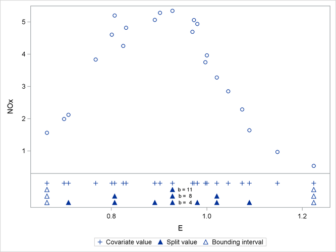
The split value for b = 11 is also a split value for b = 8, the split values for b = 8 are a subset of those for b = 4, and so forth. Figure 44.16 displays the data and the location of split values for the three cases. For a one-dimensional problem (a univariate smoother), the vertices comprise the split values and the values on the bounding interval.
You might want to move away from the boundary, in particular for an irregular data configuration or for multivariate smoothing.
The KNOTTYPE
=CENTER suboption of the KNOTMETHOD=
option chooses centroids of the leaf node cells instead of vertices. This tends to move the outer knot locations closer to
the convex hull, but not necessarily to data locations. In the emission example, choosing a bucket size of b = 11 and centroids as knot locations yields two knots at E=0.7956 and E=1.076. If you choose the NEAREST
suboption, then the nearest neighbor of a vertex or centroid will serve as the knot location. In this case, the knot locations
are a subset of the data locations, regardless of the dimension of the smooth.