The Power and Sample Size Application
Suppose you want to determine the power for a new marketing study. You want to compare car sales in the southeastern region to the national average of 1.0 car per salesperson per day. You believe that the actual average for the region is 1.6 cars per salesperson per day. You want to test if the mean for a single group is larger than a specific value, so the one-sample t test is the appropriate analysis. The conjectured mean is 1.6 and the null mean is 1.0. You intend to use a significance level of 0.05 for the one-sided test. You want to calculate power for two standard deviations, 0.5 and 0.75, and two sample sizes, 10 and 20 dealerships.
First, open a new project by selecting → on the menu bar or clicking the icon on the toolbar. The New window appears. Then, select the appropriate analysis.
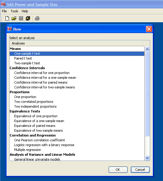
For this example, the selected analysis is the in the Means section, as shown at the top of Figure 78.2. Select the analysis from the list and click . The project window appears with the Edit Properties page displayed, as shown in Figure 78.3.
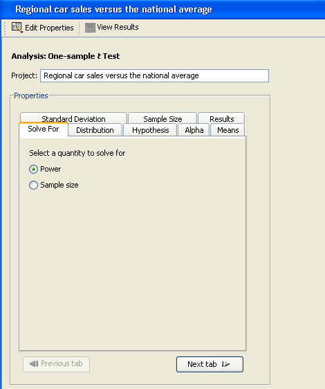
Enter a descriptive label of the project in the Project: field. For the example, change the description to Regional car sales versus the national average. The description is used to identify the project when you reopen it from the Open window.
Select → to save the description change. Note in Figure 78.3 that the title bar of the window contains your project description after you have saved the change.
Properties of the project are displayed on several tabs. You can change from tab to tab by clicking a tab or by clicking the or buttons. To display help about the properties for a tab, click the button at the bottom of the Edit Properties page.
First, click the Solve For tab and choose to calculate power or sample size. For this example, select the option, as shown in Figure 78.3.
Next, you must provide values for two analysis options and four parameters. These parameters are set in separate tabs on the Edit Properties page and are labeled Distribution, Hypothesis, Alpha, Mean, Standard Deviation, and Sample Size.
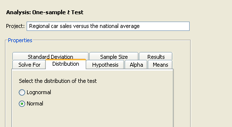
Click the Distribution tab to select a or distribution. For the example, you are using means rather than mean ratios, so select , as shown in Figure 78.4.
Click the Hypothesis tab to select a one- or two-sided test. Because you are interested only in whether the southeastern region produces higher daily car sales than the national average, select , as shown in Figure 78.5.
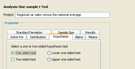
There are three one-sided test options: , , and . The option would also be appropriate for this example.
Click the Alpha tab to specify one or more significance levels. Enter 0.05, as shown in Figure 78.6.
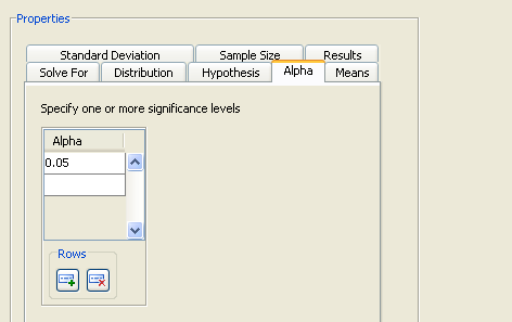
This value will be the default unless the default has been changed in the Preferences window. To set preferences, select → on the menu bar. For more information about setting preferences, see the section Setting Preferences.
Click the Means tab to enter one or more means and null means. For the example, enter 1.6 in the Mean table and 1.0 in the Null Mean table. Figure 78.7 shows the entered values.
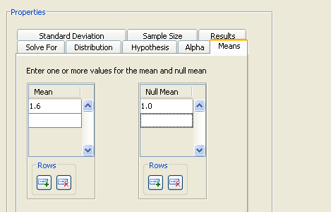
Note that additional input rows are available if you want to enter additional sets of parameters. You can also append and
delete rows using the
 and
and
 buttons beneath the table. In addition, by selecting a row and right-clicking, you can choose to insert and delete rows in
the body of the table from a pop-up menu.
buttons beneath the table. In addition, by selecting a row and right-clicking, you can choose to insert and delete rows in
the body of the table from a pop-up menu.
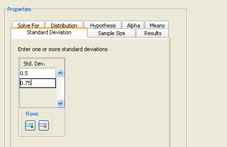
Click the Standard Deviation tab to enter standard deviations. You are interested in two standard deviations, 0.5 and 0.75. Enter them in the table, as shown in Figure 78.8.
You want to be able to sample between 10 and 20 dealerships. Click the Sample Size tab and enter these two values, as shown in Figure 78.9.
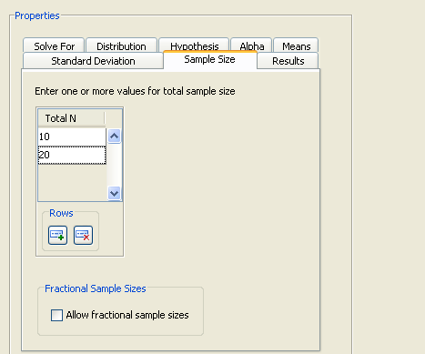
The input values are combined into one or more scenarios. In this case, each of the two standard deviations is combined with each of the two sample sizes for a total of four scenarios. Then power is computed for each scenario. In this example, only a single value or setting is present for the mean, null mean, and alpha level, so they are common to all scenarios.
Click the Results tab to select results options including a Summary Table and a Power by Sample Size graph.
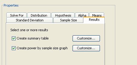
For this example, select both results check boxes: and , as shown in Figure 78.10. These selections can also be set as preferences; see the section Setting Preferences.
Click the button beside the check box to customize the graph. The Customize Graph window contains two tabs: Axis Orientation and Value Ranges, as shown in Figure 78.11.
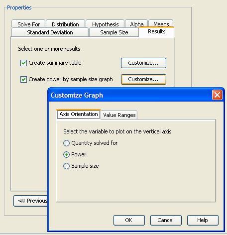
Click the Axis Orientation tab to select which quantity you would like to plot on the vertical axis. You can choose to display the quantity solved for (either power or sample size) on the vertical axis or you can choose to display power or sample size on the vertical axis with the other quantity appearing on the horizontal axis. The default is (or power) on the vertical axis, which is appropriate for this graph.
The summary table is created using the two sample sizes specified in the Sample Size table, 10 and 20. If you want to create a graph that contains more than these two sample sizes, you can do so by customizing the value ranges for the graph. Click the Value Ranges tab to set the axis range for sample sizes, as shown in Figure 78.12.
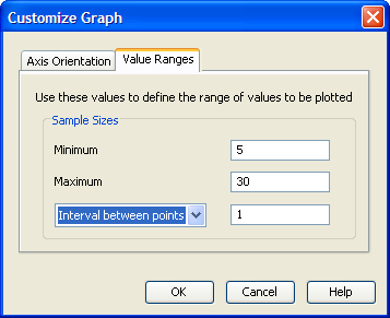
Enter 5 for the minimum and 30 for the maximum. Also, select in the drop-down list and enter a value of 1. These values set the sample size axis to range from 5 to 30 in increments of 1. The completed Value Ranges section of the
window is shown in Figure 78.12.
When you solve for power, you can set a range for sample size values, but not for the powers; and vice versa when you solve for sample size. That is, you cannot set the range of axis values for the quantity that you are solving for.
Click to save the values that you have entered and return to the Edit Properties page.
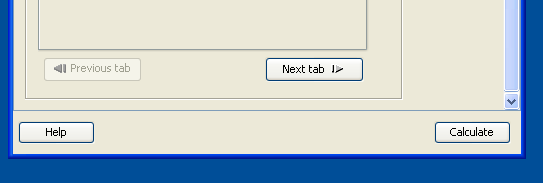
You have now specified all of the necessary input values. Click to perform the analysis, as shown in Figure 78.13.
Alternatively, you could choose to save the information that you have entered by selecting → from the menu bar or clicking the toolbar icon, and perform the analysis at another time. No error checking is done when you save the project.
You can close the project by selecting → on the menu bar or clicking the window close X in the upper right corner of the project window. You can reopen a project by selecting → on the menu bar or clicking the toolbar icon.
For this example, click .
Results appear on the View Results page and are viewable in separate tabs. The tabs include Summary Table, Graph, Narratives, SAS Log, and SAS Code (located on the left side of the View Results page). The Summary Table and Graph tabs appear if you selected those options on the Results tab of the Edit Properties page. The other tabs always appear.
Click the Summary Table tab to view the summary table.
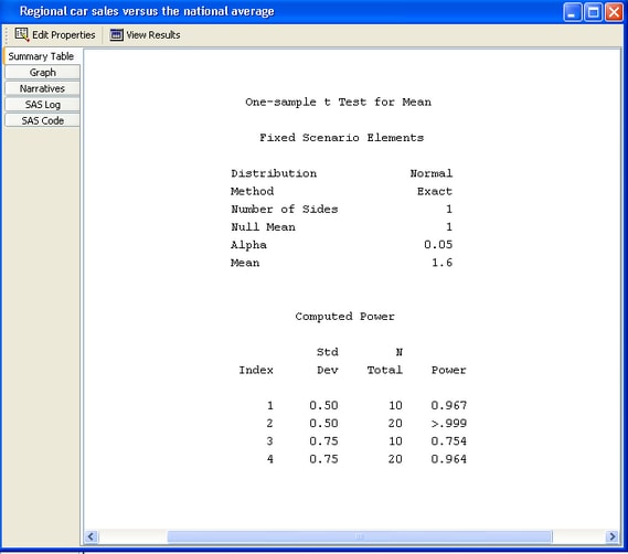
The Summary table consists of two subtables, as shown in Figure 78.14. The Fixed Scenario Elements table includes the parameters or options that have a single value for the analysis. The Computed Power table contains the input parameters that have been given more than one value, and it shows the computed quantity, power.
Thus, the Computed Power table contains four rows for the four combinations of standard deviation and sample size. From the table you can see that
all four powers are high. The smallest value of power, 0.754, is associated with the largest standard deviation and the smallest
sample size. In other words, the probability of rejecting the null hypothesis is greater than 75% in all four scenarios.
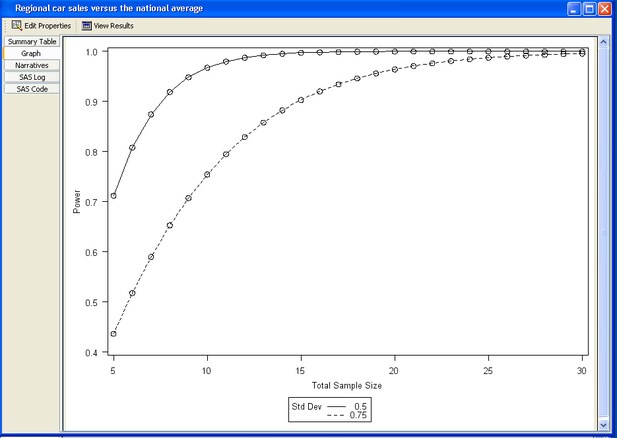
Click the Graph tab to view the power by sample size graph.
The power by sample size graph in Figure 78.15 contains one curve for each standard deviation. For a standard deviation of 0.5 (the upper curve), increasing sample size above 10 does not lead to much increase in power. If you are satisfied with a power of 0.75 or greater, 10 samples would be adequate for standard deviations between 0.5 and 0.75.
Click the Narratives tab to display a facility for creating narratives.
Narratives are descriptions of the values that compose each scenario and include a statement about the computed power or sample size.
To create narratives, choose one or more scenarios in the table at the bottom of the tab. A narrative for each selected scenario is displayed in the top portion of the tab. See Figure 78.16.
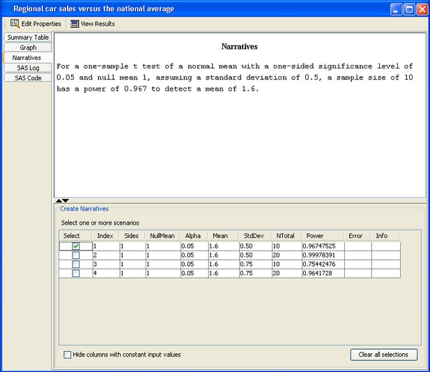
For the example, select the first row in the table. The following narrative is displayed for the scenario with a standard deviation of 0.5 and a sample size of 10:
For a one-sample t test of a normal mean with a one-sided significance level of 0.05 and null mean 1, assuming a standard deviation of 0.5, a sample size of 10 has a power of 0.967 to detect a mean of 1.6.
You can select several rows in the table. As you select each one, a corresponding narrative is created and displayed in the top portion of the table. Selecting a second scenario (the third row) produces the following output, where the narrative for the first row is followed by the narrative for the third row:
For a one-sample t test of a normal mean with a one-sided significance level of 0.05 and null mean 1, assuming a standard deviation of 0.5, a sample size of 10 has a power of 0.967 to detect a mean of 1.6. For a one-sample t test of a normal mean with a one-sided significance level of 0.05 and null mean 1, assuming a standard deviation of 0.75, a sample size of 10 has a power of 0.754 to detect a mean of 1.6.
Other results include the SAS log and the SAS code.
The SAS log that was produced when the button was last clicked appears on the SAS Log tab.
The SAS statements that produced the results appear on the SAS Code tab.
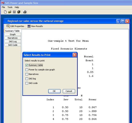
To print one or more results, select → from the menu bar or click the toolbar icon. A window is displayed that lists all available results, as shown in Figure 78.17. Select the results that you want to print and click .
If you want to change some values of the properties and rerun the analysis, change to the Edit Properties page and continue. The icons for selecting the Edit Properties and View Results pages are in the command bar just below the project window title.
When you are finished working with a project, close it by clicking the X in the upper right corner of the project window or selecting → on the menu bar. If you have not saved the project, you will be asked if you want to save it before closing.
You can reopen existing projects using the Open window. Select → on the menu bar or click the toolbar icon.
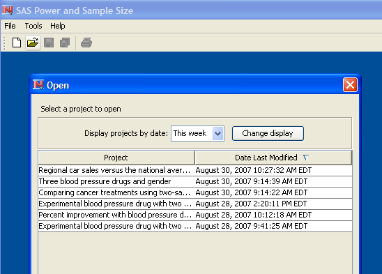
As shown in Figure 78.18, the analysis that you just completed is listed in the table. The label that you assigned to it, Regional car sales versus the national average, appears in the Project column of the table. The table also contains the date that the analysis was last modified. If you do not see the project
that you are looking for, change the value of the Display projects by date box to All by selecting All from the drop-down list, and click the button.
You can sort the projects in the table by clicking the header of the desired column. The sort direction is indicated by arrows displayed in the column header.
Select the project that you want to open and click . You can also double-click the project entry to open it.
After viewing the graph, you might want to re-create the graph with a different range for sample sizes. On the Results tab of the Edit Properties page, click the button for the power by sample size graph. The Customize Graph window is displayed.
On the Value Ranges tab of the window, change the Maximum value in the Sample Size table from 30 to 20. Click .
Rerun the analysis by clicking . The View Results page is displayed again and the graph now has the new maximum value for the sample size axis.