The QUANTSELECT Procedure

Under the iid assumption, Koenker and Machado (1999) proposed two types of quasi-likelihood ratio tests for quantile regression, where the error distribution is flexible but not limited to the asymmetric Laplace distribution. The Type I test score, LR1, is defined as
where ![]() is the sum of check losses for the reduced model,
is the sum of check losses for the reduced model, ![]() is the sum of check losses for the extended model, and
is the sum of check losses for the extended model, and ![]() is the estimated sparsity function. The Type II test score, LR2, is defined as
is the estimated sparsity function. The Type II test score, LR2, is defined as
Under the null hypothesis that the reduced model is the true model, both LR1 and LR2 follow a ![]() distribution with
distribution with ![]() degrees of freedom, where
degrees of freedom, where ![]() and
and ![]() are the degrees of freedom for the reduced model and the extended model, respectively.
are the degrees of freedom for the reduced model and the extended model, respectively.
If you specify the TEST=LR1 option in the MODEL statement, the QUANTSELECT procedure uses LR1 score to compute the significance level. Or you can use the substitutable TEST=LR2 option for computing the significance level on Type II quasi-likelihood ratio test.
Under the iid assumption, the sparsity function is defined as ![]() . Here the distribution of errors F is flexible but not limited to the asymmetric Laplace distribution. The algorithm for estimating
. Here the distribution of errors F is flexible but not limited to the asymmetric Laplace distribution. The algorithm for estimating ![]() is as follows:
is as follows:
-
Fit a quantile regression model and compute the residuals. Each residual
 can be viewed as an estimated realization of the corresponding error
  . Then
  is computed on the reduced model for testing the entry effect and on the extended model for testing the removal effect.
-
Compute quantile level bandwidth
 . The QUANTSELECT procedure computes the Bofinger bandwidth, which is an optimizer of mean squared error for standard density
estimation:
. The QUANTSELECT procedure computes the Bofinger bandwidth, which is an optimizer of mean squared error for standard density
estimation:
![\[ h_ n = n^{-1\slash 5} ( {4.5v^2(\tau )} )^{1\slash 5} \]](images/statug_qrsel0054.png)
The quantity
![\[ v(\tau ) = {\frac{s(\tau )}{s^{(2)}(\tau )}} = {\frac{f^2}{2(f^{(1)} \slash f)^2 + [(f^{(1)} \slash f)^2 - f^{(2)}\slash f ] }} \]](images/statug_qrsel0055.png)
is not sensitive to f and can be estimated by assuming f is Gaussian as
![\[ \hat{v}(\tau )={{\exp (-q^2)} \over 2\pi (q^2+1)} \mbox{ with } q=\Phi ^{-1}(\tau ) \]](images/statug_qrsel0056.png)
-
Compute residual quantiles
 and
and  as follows:
-
Set
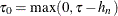 and
and 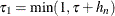 .
.
-
Use the equation
![\[ {\hat F}^{-1}(t) = \left\{ \begin{array}{ll} r_{(1)} & {\mbox{if }} t\in [0, 1\slash 2n) \\ \lambda r_{(i+1)} + (1-\lambda ) r_{(i)} & {\mbox{if }} t\in [(i-0.5)\slash n, (i+0.5)\slash n) \\ r_{(n)} & {\mbox{if }} t\in [(2n-1), 1] \\ \end{array} \right. \]](images/statug_qrsel0061.png)
where
 is the ith smallest residual and
 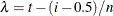 .
.
-
If
 , find i that satisfies
  and
and 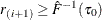 . If such an i exists, reset
  so that
  . Also find j that satisfies
  and
and 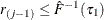 . If such a j exists, reset
  so that
  .
.
-
-
Estimate the sparsity function
 as
as
![\[ \hat{s}(\tau )={{\hat{F}^{-1}(\tau _1)-\hat{F}^{-1}(\tau _0)} \over {\tau _1-\tau _0}} \]](images/statug_qrsel0073.png)
Because a real data set might not follow the null hypothesis and the iid assumptions, the LR1 and LR2 scores that are used
for quantile regression effect selection often do not follow a ![]() distribution. Hence, the SLENTRY and SLSTAY values cannot reliably be viewed as probabilities. One way to address this difficulty
is to treat the SLENTRY and SLSTAY values only as criteria for comparing importance levels of effect candidates at each selection
step, and not to explain these values as probabilities.
distribution. Hence, the SLENTRY and SLSTAY values cannot reliably be viewed as probabilities. One way to address this difficulty
is to treat the SLENTRY and SLSTAY values only as criteria for comparing importance levels of effect candidates at each selection
step, and not to explain these values as probabilities.