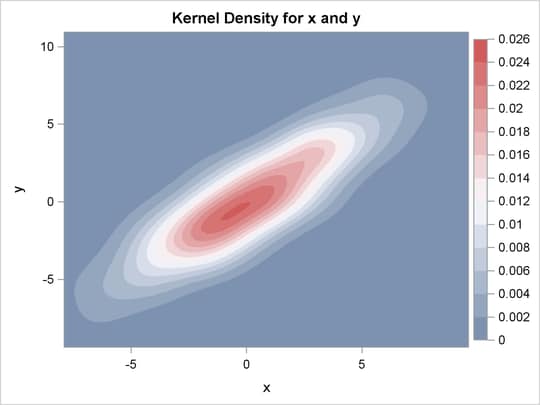
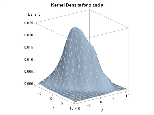
This example is taken from the section Getting Started: KDE Procedure in Chapter 52: The KDE Procedure. Here, in addition to the ODS GRAPHICS statement, procedure options are used to request plots. The following statements simulate 1,000 observations from a bivariate normal density with means (0,0), variances (10,10), and covariance 9:
data bivnormal;
   do i = 1 to 1000;
      z1 = rannor(104);
      z2 = rannor(104);
      z3 = rannor(104);
      x  = 3*z1+z2;
      y  = 3*z1+z3;
      output;
   end;
run;
The following statements request a bivariate kernel density estimate for the variables x and y:
ods graphics on;

proc kde data=bivnormal;
   bivar x y / plots=contour surface;
run;
The PLOTS= option requests a contour plot and a surface plot of the estimate (displayed in Figure 21.5 and Figure 21.6, respectively). For more information about the graphs available in PROC KDE, see the section ODS Graphics in Chapter 52: The KDE Procedure.