There are several forms of likelihood estimation and a large number of offshoot principles derived from it, such as pseudo-likelihood, quasi-likelihood, composite likelihood, etc. The basic likelihood principle is maximum likelihood, which asks to estimate the model parameters by those quantities that maximize the likelihood function of the data. The likelihood function is the joint distribution of the data, but in contrast to a probability mass or density function, it is thought of as a function of the parameters, given the data. The heuristic appeal of the maximum likelihood estimates (MLE) is that these are the values that make the observed data “most likely.” Especially for discrete response data, the value of the likelihood function is the ordinate of a probability mass function, even if the likelihood is not a probability function. Since a statistical model is thought of as a representation of the data-generating mechanism, what could be more preferable as parameter estimates than those values that make it most likely that the data at hand will be observed?
Maximum likelihood estimates, if they exist, have appealing statistical properties. Under fairly mild conditions, they are best-asymptotic-normal (BAN) estimates—that is, their asymptotic distribution is normal, and no other estimator has a smaller asymptotic variance. However, their statistical behavior in finite samples is often difficult to establish, and you have to appeal to the asymptotic results that hold as the sample size tends to infinity. For example, maximum likelihood estimates are often biased estimates and the bias disappears as the sample size grows. A famous example is random sampling from a normal distribution. The corresponding statistical model is
where the symbol ![]() is read as “is distributed as” and iid is read as “independent and identically distributed.” Under the normality assumption, the density function of
is read as “is distributed as” and iid is read as “independent and identically distributed.” Under the normality assumption, the density function of ![]() is
is
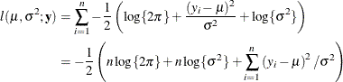
and the likelihood for a random sample of size n is
Maximizing the likelihood function ![]() is equivalent to maximizing the log-likelihood function
is equivalent to maximizing the log-likelihood function ![]() ,
,
The maximum likelihood estimators of ![]() and
and ![]() are thus
are thus
The MLE of the mean ![]() is the sample mean, and it is an unbiased estimator of
is the sample mean, and it is an unbiased estimator of ![]() . However, the MLE of the variance
. However, the MLE of the variance ![]() is not an unbiased estimator. It has bias
is not an unbiased estimator. It has bias
As the sample size n increases, the bias vanishes.
For certain classes of models, special forms of likelihood estimation have been developed to maintain the appeal of likelihood-based statistical inference and to address specific properties that are believed to be shortcomings:
-
The bias in maximum likelihood parameter estimators of variances and covariances has led to the development of restricted (or residual) maximum likelihood (REML) estimators that play an important role in mixed models.
-
Quasi-likelihood methods do not require that the joint distribution of the data be specified. These methods derive estimators based on only the first two moments (mean and variance) of the joint distributions and play an important role in the analysis of correlated data.
-
The idea of composite likelihood is applied in situations where the likelihood of the vector of responses is intractable but the likelihood of components or functions of the full-data likelihood are tractable. For example, instead of the likelihood of
 , you might consider the likelihood of pairwise differences
  .
.
-
The pseudo-likelihood concept is also applied when the likelihood function is intractable, but the likelihood of a related, simpler model is available. An important difference between quasi-likelihood and pseudo-likelihood techniques is that the latter make distributional assumptions to obtain a likelihood function in the pseudo-model. Quasi-likelihood methods do not specify the distributional family.
-
The penalized likelihood principle is applied when additional constraints and conditions need to be imposed on the parameter estimates or the resulting model fit. For example, you might augment the likelihood with conditions that govern the smoothness of the predictions or that prevent overfitting of the model.
For many statistical modeling problems, you have a choice between a least squares principle and the maximum likelihood principle. Table 3.1 compares these two basic principles.
Table 3.1: Least Squares and Maximum Likelihood
|
Criterion |
Least Squares |
Maximum Likelihood |
|---|---|---|
|
Requires specification of joint distribution of data |
No, but in order to perform confirmatory inference (tests, confidence intervals), a distributional assumption is needed, or an appeal to asymptotics. |
Yes, no progress can be made with the genuine likelihood principle without knowing the distribution of the data. |
|
All parameters of the model are estimated |
No. In the additive-error type models, least squares provides estimates of only the parameters in the mean function. The residual variance, for example, must be estimated by some other method—typically by using the mean squared error of the model. |
Yes |
|
Estimates always exist |
Yes, but they might not be unique, such as when the |
No, maximum likelihood estimates do not exist for all estimation problems. |
|
Estimators are biased |
Unbiased, provided that the model is correct—that is, the errors have zero mean. |
Often biased, but asymptotically unbiased |
|
Estimators are consistent |
Not necessarily, but often true. Sometimes estimators are consistent even in a misspecified model, such as when misspecification is in the covariance structure. |
Almost always |
|
Estimators are best linear unbiased estimates (BLUE) |
Typically, if the least squares assumptions are met. |
Not necessarily: estimators are often nonlinear in the data and are often biased. |
|
Asymptotically most efficient |
Not necessarily |
Typically |
|
Easy to compute |
Yes |
No |