This statement applies to the following SAS/STAT procedures:GENMOD, GLIMMIX, LIFEREG, LOGISTIC, MIXED, ORTHOREG, PHREG, PLM, PROBIT, SURVEYLOGISTIC, SURVEYPHREG, and SURVEYREG. It also applies to the RELIABILITY procedure in SAS/QC software.
The SLICE statement is similar to the LSMEANS statement. You use it to perform inferences on model effects that consist entirely of classification variables. With the SLICE statement, these effects must be higher-order effects of at least two classification variables. The effect is then partitioned into subsets that correspond to variables used in forming the effect. You can use the same options as you use for the LSMEANS statement to perform an analysis for the partitions. This analysis is also known as an analysis of simple effects (Winer, 1971).
By default, the interaction effect is partitioned by all main effects. For example, the following statements produce simple-effect
differences among the A levels for each level of B and simple-effect differences among the B levels for each level of A:
class a b;
model y = a b a*b;
slice a*b / diff nof;
For example, if the model-effect is a three-way interaction effect, the default output includes comparisons of the two-way interaction means.
Suppose, for example, that the interaction effect A*B is significant in your analysis and that you want to test the effect of A for each level of B. The appropriate statement is
slice A*B / sliceBy = B;
This produces an F test for each level of B that compares the equality of the levels of A.
For example, assume that in a balanced design factors A and B have a = 4 and b = 3 levels, respectively. Consider the following statements:
class a b;
model y = a b a*b;
slice a*b / sliceby=a diff;
The SLICE statement produces four F tests, one per level of A. The first of these tests is constructed by extracting the three rows that correspond to the first level of A from the coefficient matrix for the A*B interaction. Call this matrix ![]() and its rows
and its rows ![]() ,
, ![]() , and
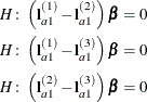
, and ![]() . The slice tests the two-degrees-of-freedom hypothesis
. The slice tests the two-degrees-of-freedom hypothesis
![\[ H\colon \left\{ \begin{array}{c} \left( \mb {l}^{(1)}_{a1} - \mb {l}^{(2)}_{a1}\right) \bbeta = 0 \\ \left( \mb {l}^{(1)}_{a1} - \mb {l}^{(3)}_{a1}\right) \bbeta = 0 \end{array} \right. \]](images/statug_introcom0249.png)
In a balanced design, where ![]() denotes the mean response if
denotes the mean response if A is at level i and B is at level j, this hypothesis is equivalent to ![]() . The DIFF option considers the three rows of
. The DIFF option considers the three rows of ![]() in turn and performs tests of the difference between pairs of rows. By default, all pairwise differences within the subset
of
in turn and performs tests of the difference between pairs of rows. By default, all pairwise differences within the subset
of ![]() are considered; in the example this corresponds to tests of the form
are considered; in the example this corresponds to tests of the form
In the example, with a = 4 and b = 3, this produces four sets of least squares means differences. Within each set, factor A is held fixed at a particular level and each set consists of three comparisons.