Loehlin (1987) points out that the models considered are unrealistic in at least two respects. First, the variables of parental aspiration, intelligence, and socioeconomic status are assumed to be measured without error. Loehlin adds uncorrelated measurement errors to the model and assumes, for illustrative purposes, that the reliabilities of these variables are known to be 0.7, 0.8, and 0.9, respectively. In practice, these reliabilities would need to be obtained from a separate study of the same or a very similar population. If these constraints are omitted, the model is not identified. However, constraining parameters to a constant in an analysis of a correlation matrix might make the chi-square goodness-of-fit test inaccurate, so there is more reason to be skeptical of the p-values. Second, the error terms for the respondent’s aspiration are assumed to be uncorrelated with the corresponding terms for his friend. Loehlin introduces a correlation between the two educational aspiration error terms and between the two occupational aspiration error terms. These additions produce the path diagram for Loehlin’s model shown in Figure 17.44.
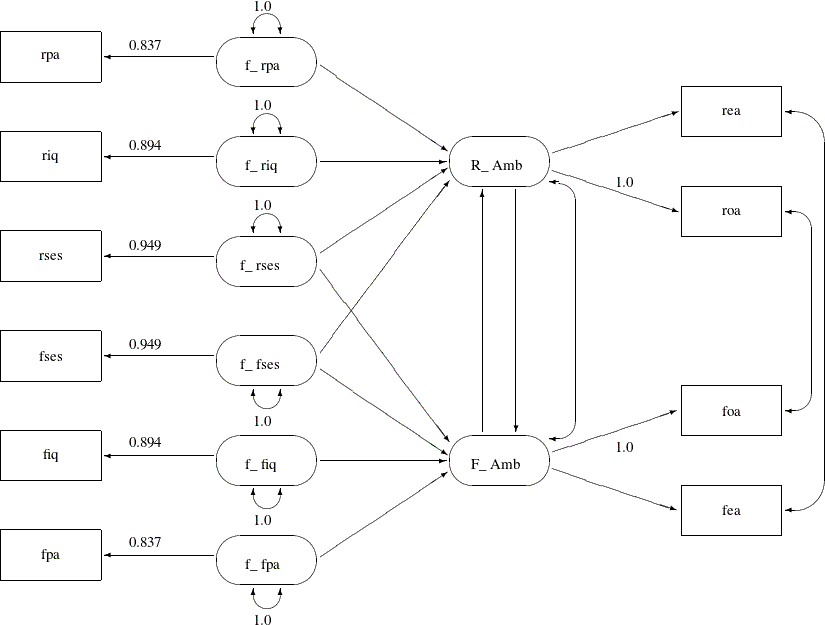
In Figure 17.44, the observed variables rpa, riq, rses, fses, fiq, and fpa are all measured with measurement errors. Their true scores counterparts f_rpa, f_riq, f_rses, f_fses, f_fiq, and f_fpa are latent variables in the model. Path coefficients from these latent variables to the observed variables are fixed coefficients,
indicating the square roots of the theoretical reliabilities in the model. These latent variables, rather than the observed
counterparts, serve as predictors of the ambition factors R_Amb and F_Amb in the current model (Analysis 3). The error terms for these two latent factors are correlated, as indicated by a double-headed
path (arrow) that connects the two factors. Correlated errors for the occupational aspiration variables (roa and foa) and the educational aspiration variables (rea and fea) are also shown in Figure 17.44. Again, these correlated errors are represented by two double-headed paths (arrows) in the path diagram.
You use the following statements to specify the path model for Analysis 3:
proc calis data=aspire nobs=329;
   path
      /* measurement model for intelligence and environment */
      rpa     <===  f_rpa    = 0.837,
      riq     <===  f_riq    = 0.894,
      rses    <===  f_rses   = 0.949,
      fses    <===  f_fses   = 0.949,
      fiq     <===  f_fiq    = 0.894,
      fpa     <===  f_fpa    = 0.837,

      /* structural model of influences */
      f_rpa   ===>  R_Amb,
      f_riq   ===>  R_Amb,
      f_rses  ===>  R_Amb,
      f_fses  ===>  R_Amb,
      f_rses  ===>  F_Amb,
      f_fses  ===>  F_Amb,
      f_fiq   ===>  F_Amb,
      f_fpa   ===>  F_Amb,
      F_Amb   ===>  R_Amb,
      R_Amb   ===>  F_Amb,

      /* measurement model for aspiration */
      R_Amb   ===>  rea        ,
      R_Amb   ===>  roa    = 1.,
      F_Amb   ===>  foa    = 1.,
      F_Amb   ===>  fea    ;
   pvar
      f_rpa f_riq f_rses f_fses f_fiq f_fpa = 6 * 1.0;
   pcov
      R_Amb F_Amb  ,
      rea  fea     ,
      roa  foa     ;
run;
In this specification, the measurement model for the six intelligence and environment variables are added. They are the first six paths in the PATH statement. Fixed constants are set for these path coefficients so as to make the measurement model identified and to set the required reliabilities of these measurement indicators. The structural model of influences and the measurement model for aspiration are the same as specified in Analysis 1. (See the section Career Aspiration: Analysis 1.) All the correlated errors are specified in the PCOV statement.
The fit summary of the current model is displayed in Figure 17.45.
Figure 17.45: Career Aspiration Data: Fit Summary for Analysis 3
| Fit Summary | |
|---|---|
| Chi-Square | 12.0132 |
| Chi-Square DF | 13 |
| Pr > Chi-Square | 0.5266 |
| Standardized RMR (SRMR) | 0.0149 |
| Adjusted GFI (AGFI) | 0.9692 |
| RMSEA Estimate | 0.0000 |
| Akaike Information Criterion | 96.0132 |
| Schwarz Bayesian Criterion | 255.4476 |
| Bentler Comparative Fit Index | 1.0000 |
Since the p-value for the chi-square test is 0.5266, this model clearly cannot be rejected. Both the standardized RMSR and the RMSEA are very small, and both the adjusted GFI and the comparative fit index are high. All these point to an excellent model fit. However, Schwarz’s Bayesian criterion for this model (SBC = 255.4476) is somewhat larger than for Jöreskog and Sörbom (1988) Analysis 2 in Figure 17.42 (SBC = 247.1489), suggesting that a more parsimonious model would be desirable.
The estimation results are displayed in Figure 17.46.
Figure 17.46: Career Aspiration Data: Estimation Results for Analysis 3
| PATH List | ||||||
|---|---|---|---|---|---|---|
| Path | Parameter | Estimate | Standard Error |
t Value | ||
| rpa | <=== | f_rpa | 0.83700 | |||
| riq | <=== | f_riq | 0.89400 | |||
| rses | <=== | f_rses | 0.94900 | |||
| fses | <=== | f_fses | 0.94900 | |||
| fiq | <=== | f_fiq | 0.89400 | |||
| fpa | <=== | f_fpa | 0.83700 | |||
| f_rpa | ===> | R_Amb | _Parm01 | 0.18370 | 0.05044 | 3.64197 |
| f_riq | ===> | R_Amb | _Parm02 | 0.28004 | 0.06139 | 4.56182 |
| f_rses | ===> | R_Amb | _Parm03 | 0.22616 | 0.05223 | 4.32999 |
| f_fses | ===> | R_Amb | _Parm04 | 0.08698 | 0.05476 | 1.58829 |
| f_rses | ===> | F_Amb | _Parm05 | 0.06327 | 0.05219 | 1.21242 |
| f_fses | ===> | F_Amb | _Parm06 | 0.21539 | 0.05121 | 4.20597 |
| f_fiq | ===> | F_Amb | _Parm07 | 0.35387 | 0.06741 | 5.24970 |
| f_fpa | ===> | F_Amb | _Parm08 | 0.16876 | 0.04934 | 3.42048 |
| F_Amb | ===> | R_Amb | _Parm09 | 0.11898 | 0.11396 | 1.04412 |
| R_Amb | ===> | F_Amb | _Parm10 | 0.13022 | 0.12067 | 1.07912 |
| R_Amb | ===> | rea | _Parm11 | 1.08399 | 0.09417 | 11.51051 |
| R_Amb | ===> | roa | 1.00000 | |||
| F_Amb | ===> | foa | 1.00000 | |||
| F_Amb | ===> | fea | _Parm12 | 1.11630 | 0.08627 | 12.93945 |
| Variance Parameters | |||||
|---|---|---|---|---|---|
| Variance Type |
Variable | Parameter | Estimate | Standard Error |
t Value |
| Exogenous | f_rpa | 1.00000 | |||
| f_riq | 1.00000 | ||||
| f_rses | 1.00000 | ||||
| f_fses | 1.00000 | ||||
| f_fiq | 1.00000 | ||||
| f_fpa | 1.00000 | ||||
| Error | riq | _Add01 | 0.20874 | 0.07832 | 2.66518 |
| rpa | _Add02 | 0.29584 | 0.07774 | 3.80572 | |
| rses | _Add03 | 0.09887 | 0.07803 | 1.26712 | |
| roa | _Add04 | 0.42307 | 0.05243 | 8.06949 | |
| rea | _Add05 | 0.32707 | 0.05452 | 5.99881 | |
| fiq | _Add06 | 0.19989 | 0.07674 | 2.60483 | |
| fpa | _Add07 | 0.29988 | 0.07807 | 3.84092 | |
| fses | _Add08 | 0.10324 | 0.07824 | 1.31952 | |
| foa | _Add09 | 0.42240 | 0.04730 | 8.93099 | |
| fea | _Add10 | 0.28716 | 0.04804 | 5.97756 | |
| R_Amb | _Add11 | 0.25418 | 0.04469 | 5.68740 | |
| F_Amb | _Add12 | 0.19698 | 0.03814 | 5.16528 | |
| Covariances Among Exogenous Variables | |||||
|---|---|---|---|---|---|
| Var1 | Var2 | Parameter | Estimate | Standard Error |
t Value |
| f_riq | f_rpa | _Add13 | 0.24677 | 0.07519 | 3.28202 |
| f_rses | f_rpa | _Add14 | 0.06183 | 0.06945 | 0.89030 |
| f_rses | f_riq | _Add15 | 0.26351 | 0.06687 | 3.94078 |
| f_fses | f_rpa | _Add16 | 0.02382 | 0.06952 | 0.34267 |
| f_fses | f_riq | _Add17 | 0.22136 | 0.06648 | 3.32983 |
| f_fses | f_rses | _Add18 | 0.30156 | 0.06359 | 4.74210 |
| f_fiq | f_rpa | _Add19 | 0.10853 | 0.07362 | 1.47416 |
| f_fiq | f_riq | _Add20 | 0.42476 | 0.07219 | 5.88372 |
| f_fiq | f_rses | _Add21 | 0.27250 | 0.06660 | 4.09143 |
| f_fiq | f_fses | _Add22 | 0.34922 | 0.06771 | 5.15762 |
| f_fpa | f_rpa | _Add23 | 0.15789 | 0.07873 | 2.00555 |
| f_fpa | f_riq | _Add24 | 0.13084 | 0.07418 | 1.76387 |
| f_fpa | f_rses | _Add25 | 0.11516 | 0.06978 | 1.65050 |
| f_fpa | f_fses | _Add26 | -0.05622 | 0.06971 | -0.80648 |
| f_fpa | f_fiq | _Add27 | 0.27867 | 0.07530 | 3.70082 |
| Covariances Among Errors | |||||
|---|---|---|---|---|---|
| Error of | Error of | Parameter | Estimate | Standard Error |
t Value |
| R_Amb | F_Amb | _Parm13 | -0.00936 | 0.05010 | -0.18673 |
| rea | fea | _Parm14 | 0.02308 | 0.03139 | 0.73545 |
| roa | foa | _Parm15 | 0.11206 | 0.03258 | 3.43988 |
Like Analyses 1 and 2, two paths that concern the validity of the indicators in the current analysis do not show significance.
That is, f_fses does not seem to be a good indicator of a respondent’s ambition R_Amb, and f_rses does not seem to be a good indicator of a friend’s ambition F_Amb. The t values are 1.588 and 1.212, respectively. In addition, in the current model (Analysis 3), the structural relationships between
the ambition factors do not show significance. The t value for the path from the friend’s ambition factor F_Amb on the respondent’s ambition factor R_Amb is only 1.044, while the t value for the path from the respondent’s ambition factor R_Amb on the friend’s ambition factor F_Amb is only 1.079. These cast doubts on the validity of the structural model and perhaps even the entire model.