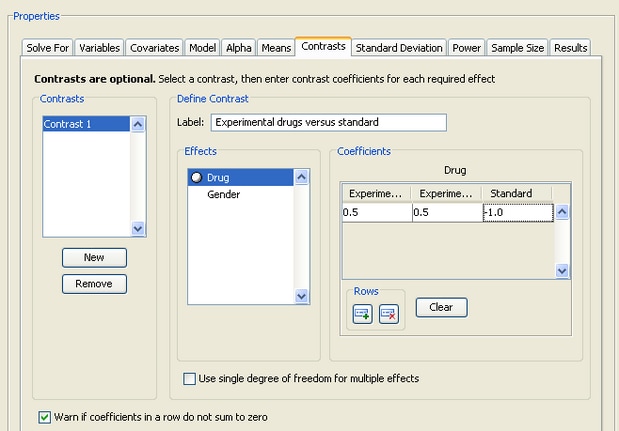
Click the Contrasts tab to define one or more contrasts. Contrasts are optional. PSS allows contrasts to be added when using either a main effects model or a main effects and interactions model. At least two factors must have been specified in order to be able to enter contrasts. The contrast tab appears in Figure 76.70.
To create a contrast, click the button. Then, select the newly created contrast (Contrast 1) from the list.
Specify a label for the contrast in the Label field. The label should be different from all of the factor names and all interactions in the model, as well as other contrast labels.
Then, for each term you want to include in the contrast, select the term in the list and enter at least two coefficients per term. It is not necessary to enter zeros; blanks are considered to be zeros.
To clear all of the contrast coefficients for a term, click the button. To remove a previously defined contrast, select it from the list and click the button.
In this example, you are interested in comparing the two experimental drugs to the standard drug. As shown in Figure 76.70, the contrast coefficients are 0.5, 0.5, and –1 for the three levels of the Drug effect.
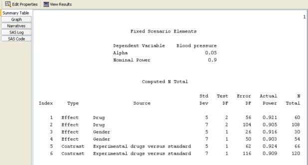
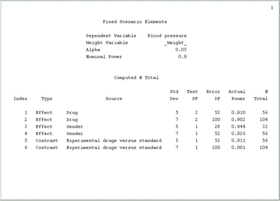
Figure 76.71 shows the two scenarios for the contrast at the bottom of the Computed N Total table. The two scenarios also appear in the graph but the graph is not shown here.
Click the Sample Size tab to select the equal or unequal cell sizes option.
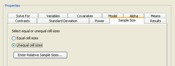
For the example, select the option, as seen in Figure 76.72, and then click the button.
Figure 76.73 shows the window in which you can enter relative sample sizes. As an example, enter the sample size weights from Table 76.8.
Table 76.8: Sample Size Weights
|
Drug |
|||
|---|---|---|---|
|
Gender |
Experimental 1 |
Experimental 2 |
Standard |
|
Males |
1 |
1 |
2 |
|
Females |
1 |
1 |
2 |
If you have unequal cell sizes, you must enter relative sample size weights for the cells. Weights do not have to sum to 1 across the cells. Some weights can be zero, but enough weights must be greater than zero so that the effects and contrasts are estimable.
In this case, you want the sample size of the standard group to be twice that of each of the two experimental groups. Click to save the values and return to the Edit Properties page.
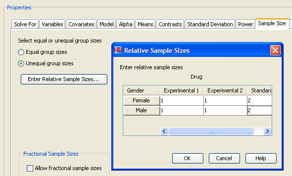
Figure 76.74 shows the summary table for the Drug by Gender example.
In addition to solving for sample size, you can also solve for power. Figure 76.75 shows the two options. Click the Solve For tab to select the option.
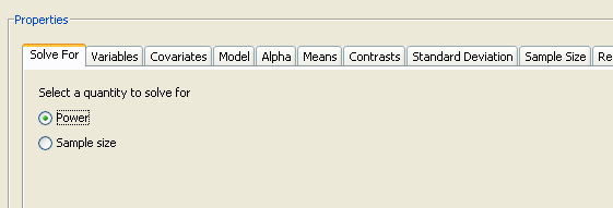
When solving for power, you must provide sample size information. For the general linear univariate model analysis, you provide
this information by using one of two alternate forms. To choose the desired alternate form, select the desired form from the
Select a form list box on the Sample Size tab. The alternate forms are:
-
Enter the sample size for a cell. Cell sizes are assumed to be equal. Sample size is reported in the summary table as total sample size.
-
Enter the total sample size and specify whether cell sizes are to be equal or unequal. Select the or option. For unequal cell sizes, you also enter cell weights. Click the button to display a window that is used to enter the data. For more information about using unequal cell sizes, see the section Using Unequal Cell Sizes.
Click the Model tab to select from three types of models: a model, a model, and a .
To specify a custom model, select the option; then a model building facility is displayed.
The facility displays a list of the factors on the left. Construct the desired model using the , , and buttons. The example shown in Figure 76.76 has the three main effects and one of the four possible interactions.
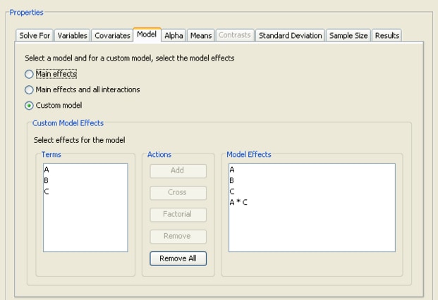
Add the three main effects (A, B, C) by selecting them in the list and clicking the button. Add the A*B interaction by selecting the A and B factors in the list and clicking the button.
To create the complete factorial design of several factors, select the factors in the list, then click the button. All possible main effects and interactions are added to the list.
To remove effects, select them in the list and click the button. Clicking the button removes all effects in the model.
Click the Covariates tab to enter covariate information.
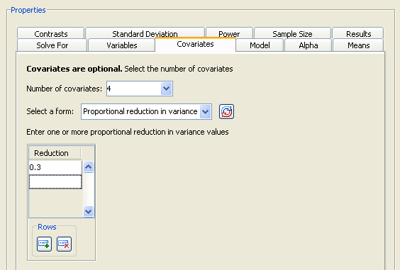
Figure 76.77 illustrates four covariates and a proportional reduction in variation of 0.3. The results for the analysis are not shown.
Covariates are optional. If you have covariates, include the total number of degrees of freedom for all covariates. To do
this, add the number of continuous covariates and the sum of the degrees of freedom of the classification covariates, and
enter this total in the Number of Covariates list box. For example, with two continuous covariates and a single classification covariate factor with three levels, the
total would be ![]() .
.
Also, you must enter the correlation between the dependent variable and the set of covariates. Two alternate forms are available: and . Select the desired form and enter one or more values.
The multiple correlation is between the set of covariates and the dependent variable. Proportional reduction in variation is how much the variance of the dependent variable is reduced by the inclusion of the covariates, expressed as a proportion between 0 and 1.