The following step runs PROC REG to fit a simple regression model and creates Output 22.2.2 and Output 22.2.1:
ods graphics on;
ods trace on;

proc reg data=sashelp.class;
   model weight = height;
run;
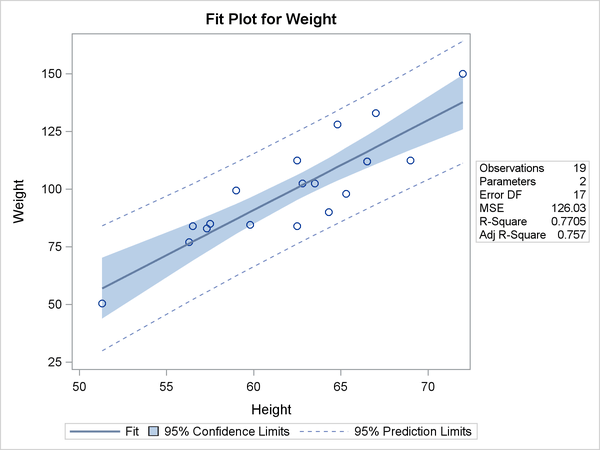
Output 22.2.1: PROC REG Output
| Number of Observations Read | 19 |
|---|---|
| Number of Observations Used | 19 |
| Analysis of Variance | |||||
|---|---|---|---|---|---|
| Source | DF | Sum of Squares |
Mean Square |
F Value | Pr > F |
| Model | 1 | 7193.24912 | 7193.24912 | 57.08 | <.0001 |
| Error | 17 | 2142.48772 | 126.02869 | ||
| Corrected Total | 18 | 9335.73684 | |||
| Root MSE | 11.22625 | R-Square | 0.7705 |
|---|---|---|---|
| Dependent Mean | 100.02632 | Adj R-Sq | 0.7570 |
| Coeff Var | 11.22330 |
| Parameter Estimates | |||||
|---|---|---|---|---|---|
| Variable | DF | Parameter Estimate |
Standard Error |
t Value | Pr > |t| |
| Intercept | 1 | -143.02692 | 32.27459 | -4.43 | 0.0004 |
| Height | 1 | 3.89903 | 0.51609 | 7.55 | <.0001 |
The fit statistics table following the “Analysis of Variance” table displays the R square and the mean. The last table displays the parameter estimates. This information is produced and processed for inclusion in the fit plot as follows:
proc reg data=sashelp.class;
   ods output fitstatistics=fs ParameterEstimates=c;
   model weight = height;
run;

data _null_;
   set fs;
   if _n_ = 1 then call symputx('R2'  , put(nvalue2, 4.2)   , 'G');
   if _n_ = 2 then call symputx('mean', put(nvalue1, best6.), 'G');
run;
data _null_;
   set c;
   length s $ 200;
   retain s ' ';
   if _n_ = 1 then
      s = trim(dependent) || ' = ' ||             /* dependent =             */
          put(estimate, best5. -L);               /* intercept               */
   else if abs(estimate) > 1e-8 then do;          /* skip zero coefficients  */
      s = trim(s) || ' ' ||                       /* string so far           */
          scan('+ -', 1 + (estimate < 0), ' ')    /* + (add) or - (subtract) */
          || ' ' ||
          trim(put(abs(estimate), best5. -L))     /* abs(coefficient)        */
          || ' ' || variable;                     /* variable name           */
   end;                                           /* e for error added next  */
   call symputx('formula', trim(s) || ' + e', 'G');
run;
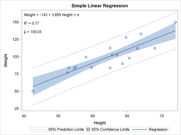
Two SAS data sets are made from the tabular output, and the R square, mean, and equation for the regression model are stored in macro variables. The following step uses PROC SGPLOT with an INSET statement to display the linear fit plot along with the R square, mean, and equation for the regression model:
proc sgplot data=sashelp.class;
   title 'Simple Linear Regression';
   inset "&formula"
         "R(*ESC*){sup '2'} = &r2"
         "(*ESC*){unicode mu}(*ESC*){unicode hat} = &mean" / position=topleft;
    reg y=weight x=height / clm cli;
run;
The results are displayed in Output 22.2.3.
Each separate string in the INSET statement is displayed in a separate line. The first string is the formula, which is generated
in the second DATA step. The next string is the R square, and it consists of an 'R', an escaped superscript 2, and the value
of R square (which is stored in a macro variable). The string for the mean consists of two Unicode specifications, one for
the Greek letter ![]() , and one to put a hat over it. These special character specifications appear in quotes and are escaped with
, and one to put a hat over it. These special character specifications appear in quotes and are escaped with (*ESC*) so that they are processed as special characters rather than as literal text. Typically, you must escape special characters
in quotes, and not escape them when they are not in quotes. See the section Unicode and Special Characters for a list of a few of the more commonly used Unicode characters.
The same information can be added to the graph that PROC REG produces by adding the following statements to the PROC REG template for a fit plot:
mvar formula;

layout gridded / autoalign=(topleft topright bottomleft
                            bottomright);
   entry halign=left formula;
   entry halign=left "R"{sup '2'} " = " eval(put(_rsquare, 4.2));
   entry halign=left "(*ESC*){unicode mu}(*ESC*){unicode hat} = "
         eval(put(_depmean, best6.))
         / textattrs=GraphValueText
                     (family=GraphUnicodeText:FontFamily);
   endlayout;
The MVAR statement names macro variables whose values are added to the graph. The MVAR statement is added to the PROC REG
fit plot template near the top. The LAYOUT GRIDDED block creates a table that consists of the equation, R square, and mean.
The LAYOUT GRIDDED block is added to the PROC REG fit plot template inside the LAYOUT OVERLAY. The option autoalign=(topleft topright bottomleft bottomright) is used to position the table in a part of the graph that is open, first trying the top left corner.
In this example, in the LAYOUT GRIDDED block, two dynamic variables for R square, and the mean are used instead of the macro
variables that were made in previous steps. The origin of the names of the two dynamic variables that are used in this example
are revealed in the next step when the source code for the PROC REG fit plot is displayed. The first ENTRY statement creates
a text line for the formula and left-justifies it. The second ENTRY statement creates the R square line. It consists of a
literal 'R', a specification for a superscript of 2 (
), an equal sign surrounded by spaces, and the formatted value of the dynamic variable with the R square. The third ENTRY
statement creates the mean line. It consists of two Unicode specifications, one for the Greek letter ![]() sup 2
sup 2
![]()
![]() , and one to put a hat over it. These special character specifications appear in quotes (unlike the
, and one to put a hat over it. These special character specifications appear in quotes (unlike the
) and are escaped with ![]() sup 2
sup 2
![]()
(*ESC*) so that they are processed as special characters rather than as literal text. Typically, you must escape special characters
in quotes, and not escape them when they are not in quotes. Note that sup along with sub (subscript) must not appear in quotes in the GTL, but they can appear in quotes in PROC SGPLOT (as was previously shown).
The option textattrs=GraphValueText (family=GraphUnicodeText:FontFamily) is specified to ensure that a font that recognizes Unicode characters is used. See the section Unicode and Special Characters for a list of a few of the more commonly used Unicode characters.
You can use the trace information from the PROC REG step (not shown) and the following step to display the template for the fit plot:
proc template;
   source Stat.Reg.Graphics.Fit;
run;
Some of the results are as follows:
define statgraph Stat.Reg.Graphics.Fit;
   notes "Fit Plot";
   dynamic _DEPLABEL _DEPNAME _MODELLABEL _SHOWSTATS _NSTATSCOLS _SHOWNObs
      _SHOWTOTFREQ _SHOWNParm _SHOWEDF _SHOWMSE _SHOWRSquare _SHOWAdjRSq
      _SHOWSSE _SHOWDepMean _SHOWCV _SHOWAIC _SHOWBIC _SHOWCP _SHOWGMSEP
      _SHOWJP _SHOWPC _SHOWSBC _SHOWSP _NObs _NParm _EDF _MSE _RSquare
      _AdjRSq _SSE _DepMean _CV _AIC _BIC _CP _GMSEP _JP _PC _SBC _SP
      _PREDLIMITS _CONFLIMITS _XVAR _SHOWCLM _SHOWCLI _WEIGHT _SHORTXLABEL
      _SHORTYLABEL _TITLE _TOTFreq;
   BeginGraph;
      entrytitle halign=left textattrs=GRAPHVALUETEXT _MODELLABEL
         halign=center textattrs=GRAPHTITLETEXT _TITLE " for " _DEPNAME;
      layout Overlay / yaxisopts=(label=_DEPLABEL shortlabel=_SHORTYLABEL)
         xaxisopts=(shortlabel=_SHORTXLABEL);
               .
               .
               .
               if (_SHOWRSQUARE^=0)
                  entry halign=left "R-Square" / valign=top;
                  entry halign=right eval (PUT(_RSQUARE,BEST6.)) / valign=top;
               endif;
               .
               .
               .
               if (_SHOWDEPMEAN^=0)
                  entry halign=left "Dependent Mean" / valign=top;
                  entry halign=right eval (PUT(_DEPMEAN,BEST6.)) / valign=top;
               endif;
               .
               .
               .
         endif;
      endlayout;
   EndGraph;
end;
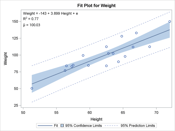
The preceding results show that the dynamic variables _RSquare and _DepMean contain the R square and the mean of the dependent variable. The MVAR statement and the LAYOUT GRIDDED block can be added
to the template, and in the interest of maximizing graph size, the table of statistics can be removed, creating the following
template:
proc template;
   define statgraph Stat.Reg.Graphics.Fit;
      notes "Fit Plot";
      mvar formula;
      dynamic _DEPLABEL _DEPNAME _MODELLABEL _SHOWSTATS _NSTATSCOLS _SHOWNObs
         _SHOWTOTFREQ _SHOWNParm _SHOWEDF _SHOWMSE _SHOWRSquare _SHOWAdjRSq
         _SHOWSSE _SHOWDepMean _SHOWCV _SHOWAIC _SHOWBIC _SHOWCP _SHOWGMSEP
         _SHOWJP _SHOWPC _SHOWSBC _SHOWSP _NObs _NParm _EDF _MSE _RSquare
         _AdjRSq _SSE _DepMean _CV _AIC _BIC _CP _GMSEP _JP _PC _SBC _SP
         _PREDLIMITS _CONFLIMITS _XVAR _SHOWCLM _SHOWCLI _WEIGHT _SHORTXLABEL
         _SHORTYLABEL _TITLE _TOTFreq;
      BeginGraph;
         entrytitle halign=left textattrs=GRAPHVALUETEXT _MODELLABEL
            halign=center textattrs=GRAPHTITLETEXT _TITLE " for " _DEPNAME;
         layout Overlay / yaxisopts=(label=_DEPLABEL shortlabel=_SHORTYLABEL)
            xaxisopts=(shortlabel=_SHORTXLABEL);
            if (_SHOWCLM=1)
               BANDPLOT limitupper=UPPERCLMEAN limitlower=LOWERCLMEAN x=_XVAR /
                  fillattrs=GRAPHCONFIDENCE connectorder=axis name="Confidence"
                  LegendLabel=_CONFLIMITS;
            endif;
            layout gridded / autoalign=(topleft topright bottomleft
                                        bottomright);
               entry halign=left formula;
               entry halign=left "R"{sup '2'} " = "  eval(put(_rsquare, 4.2));
               entry halign=left "(*ESC*){unicode mu}(*ESC*){unicode hat} = "
                     eval(put(_depmean, best6.))
                     / textattrs=GraphValueText
                                 (family=GraphUnicodeText:FontFamily);
               endlayout;
            if (_SHOWCLI=1)
               if (_WEIGHT=1)
                  SCATTERPLOT y=PREDICTEDVALUE x=_XVAR / markerattrs=(size=0)
                     datatransparency=.6 yerrorupper=UPPERCL yerrorlower=LOWERCL
                     name="Prediction" LegendLabel=_PREDLIMITS;
               else
                  BANDPLOT limitupper=UPPERCL limitlower=LOWERCL x=_XVAR /
                     display=(outline) outlineattrs=GRAPHPREDICTIONLIMITS
                     connectorder=axis name="Prediction"
                     LegendLabel=_PREDLIMITS;
               endif;
            endif;
            SCATTERPLOT y=DEPVAR x=_XVAR / markerattrs=GRAPHDATADEFAULT primary=
               true rolename=(_tip1=OBSERVATION _id1=ID1 _id2=ID2 _id3=ID3 _id4=
               ID4 _id5=ID5) tip=(y x _tip1 _id1 _id2 _id3 _id4 _id5);
            SERIESPLOT y=PREDICTEDVALUE x=_XVAR / lineattrs=GRAPHFIT
               connectorder=xaxis name="Fit" LegendLabel="Fit";
            if (_SHOWCLI=1 OR _SHOWCLM=1)
               DISCRETELEGEND "Fit" "Confidence" "Prediction" / across=3 HALIGN=
                  CENTER VALIGN=BOTTOM;
            endif;
         endlayout;
      EndGraph;
   end;
run;
The following step uses the modified template to create Output 22.2.4:
proc reg data=sashelp.class;
   model weight = height;
run;
You can restore the default template by running the following step:
proc template;
   delete Stat.Reg.Graphics.Fit / store=sasuser.templat;
run;