To see how various clustering methods differ, you must examine a more difficult problem than that of the previous example.
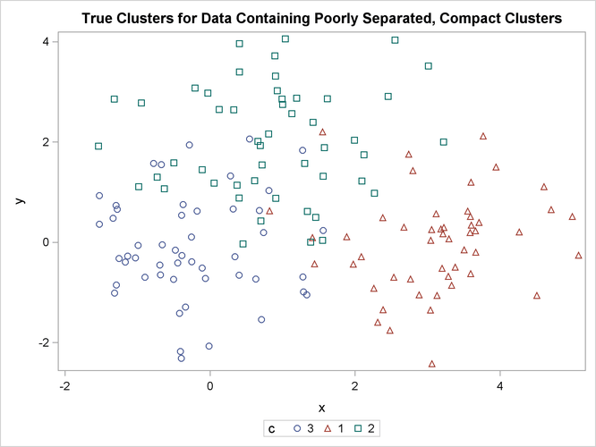
The following data set is similar to the first except that the three clusters are much closer together. This example demonstrates the use of PROC FASTCLUS and five hierarchical methods available in PROC CLUSTER. To help you compare methods, this example plots true, generated clusters. Also included is a bubble plot of the density estimates obtained in conjunction with two-stage density linkage in PROC CLUSTER.
The following SAS statements produce Figure 11.2:
data closer;
   keep x y c;
   n=50; scale=1;
   mx=0; my=0; c=3; link generate;
   mx=3; my=0; c=1; link generate;
   mx=1; my=2; c=2; link generate;
   stop;
generate:
   do i=1 to n;
      x=rannor(9)*scale+mx;
      y=rannor(9)*scale+my;
      output;
   end;
   return;
run;
title 'True Clusters for Data Containing Poorly Separated, Compact Clusters';
proc sgplot;
   scatter y=y x=x / group=c ;
run;
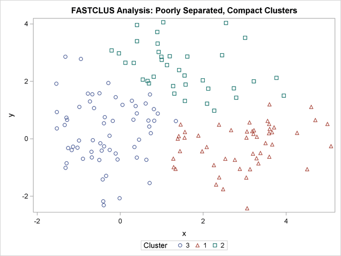
The following statements use the FASTCLUS procedure to find three clusters and then use the SGPLOT procedure to plot the clusters. The following statements produce Figure 11.3:
proc fastclus data=closer out=out maxc=3 noprint;
   var x y;
   title 'FASTCLUS Analysis: '
         'Poorly Separated, Compact Clusters';
run;

proc sgplot;
   scatter y=y x=x / group=cluster;
run;
The following SAS statements produce Figure 11.4:
proc cluster data=closer outtree=tree method=ward noprint;
   var x y;
run;

proc tree noprint out=out n=3;
   copy x y;
   title 'Ward''s Minimum Variance Cluster Analysis: '
         'Poorly Separated, Compact Clusters';
run;

proc sgplot;
   scatter y=y x=x / group=cluster;
run;
The following SAS statements produce Figure 11.5:
proc cluster data=closer outtree=tree method=average noprint;
   var x y;
run;

proc tree noprint out=out n=3 dock=5;
   copy x y;
   title 'Average Linkage Cluster Analysis: '
         'Poorly Separated, Compact Clusters';
run;

proc sgplot;
   scatter y=y x=x / group=cluster;
run;
The following SAS statements produce Figure 11.6:
proc cluster data=closer outtree=tree method=centroid noprint;
var x y;
run;
proc tree noprint out=out n=3 dock=5;
copy x y;
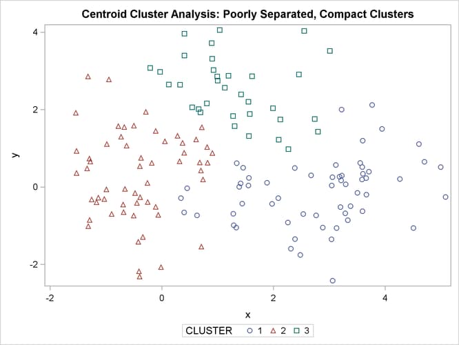
title 'Centroid Cluster Analysis: '
'Poorly Separated, Compact Clusters';
run;
proc sgplot;
scatter y=y x=x / group=cluster;
run;
The following SAS statements produce Figure 11.7 and Figure 11.8:
proc cluster data=closer outtree=tree method=twostage k=10 noprint;
   var x y;
run;

proc tree noprint out=out n=3;
   copy x y _dens_;
   title 'Two-Stage Density Linkage Cluster Analysis: '
         'Poorly Separated, Compact Clusters';
run;

proc sgplot;
   scatter y=y x=x / group=cluster;
run;
proc sgplot;
   bubble y=y x=x size=_dens_ / nofill lineattrs=graphdatadefault;
   title 'Estimated Densities for Data Containing Poorly Separated, '
         'Compact Clusters';
run;
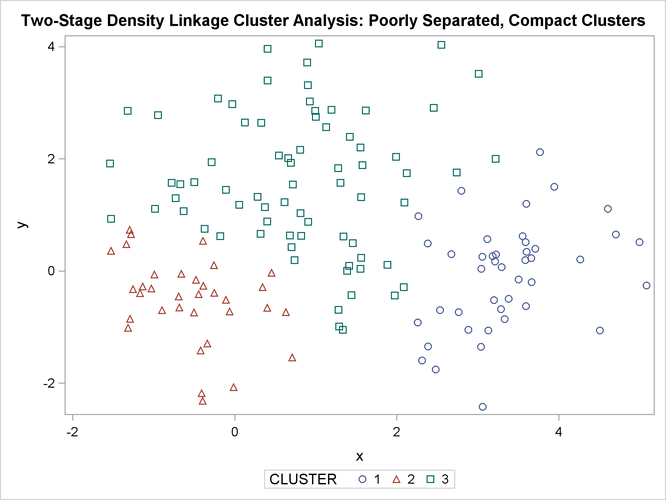
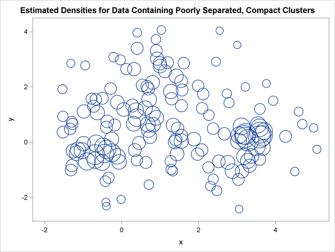
In two-stage density linkage, each cluster is a region surrounding a local maximum of the estimated probability density function. If you think of the estimated density function as a landscape with mountains and valleys, each mountain is a cluster, and the boundaries between clusters are placed near the bottoms of the valleys.
The following SAS statements produce Figure 11.9:
proc cluster data=closer outtree=tree method=single noprint;
   var x y;
run;

proc tree data=tree noprint out=out n=3 dock=5;
   copy x y;
   title 'Single Linkage Cluster Analysis: '
         'Poorly Separated, Compact Clusters';
run;

proc sgplot;
   scatter y=y x=x / group=cluster;
run;
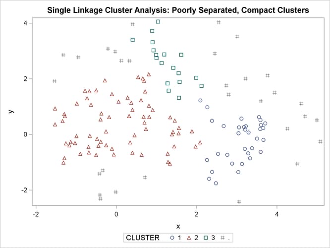
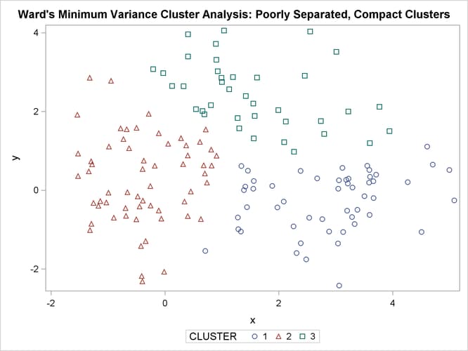
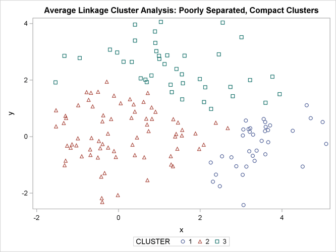
The two least squares methods, PROC FASTCLUS and Ward’s, yield the most uniform cluster sizes and the best recovery of the true clusters. This result is expected since these two methods are biased toward recovering compact clusters of equal size. With average linkage, the lower-left cluster is too large; with the centroid method, the lower-right cluster is too large; and with two-stage density linkage, the top cluster is too large. The single linkage analysis resembles average linkage except for the large number of outliers resulting from the DOCK= option in the PROC TREE statement; the outliers are plotted as filled circles (missing values).