The FMM Procedure

It is important to note that Roeder’s original analysis proceeds in a different manner than the finite mixture modeling presented here. The technique presented by Roeder first develops a “best” range of scale parameters based on a specific criterion. Roeder then uses fixed scale parameters taken from this range to develop optimal equal-scale Gaussian mixture models.
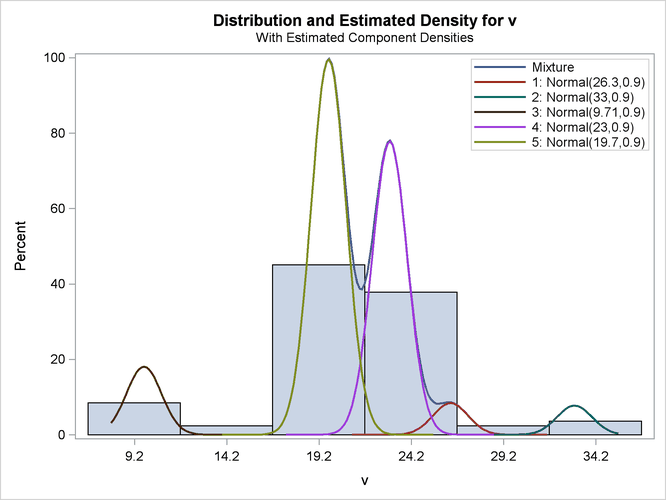
You can reproduce Roeder’s point estimate for the density by specifying a five-component Gaussian mixture. In addition, use
the EQUATE=SCALE option in the MODEL statement and a RESTRICT statement fixing the first component’s scale parameter at 0.9025 (Roeder’s h = 0.95, scale![]() ). The combination of these options produces a mixture of five Gaussian components, each with variance 0.9025. The following
statements conduct this analysis:
). The combination of these options produces a mixture of five Gaussian components, each with variance 0.9025. The following
statements conduct this analysis:
title2 "Five Components, Equal Variances = 0.9025";
ods select DensityPlot;
proc fmm data=galaxies;
   model v = / K=5 equate=scale;
   restrict int 0 (scale 1) = 0.9025;
   ods exclude IterHistory OptInfo ComponentInfo;
run;
ods graphics off;
The output is shown in Figure 37.18 and Figure 37.19.
Figure 37.18: Reproduction of Roeder’s Five-Component Analysis of Galaxy Data
| FMM Analysis of Galaxies Data |
| Five Components, Equal Variances = 0.9025 |
| Model Information | |
|---|---|
| Data Set | WORK.GALAXIES |
| Response Variable | v |
| Type of Model | Homogeneous Mixture |
| Distribution | Normal |
| Components | 5 |
| Link Function | Identity |
| Estimation Method | Maximum Likelihood |
| Fit Statistics | |
|---|---|
| -2 Log Likelihood | 412.2 |
| AIC (smaller is better) | 430.2 |
| AICC (smaller is better) | 432.7 |
| BIC (smaller is better) | 451.9 |
| Pearson Statistic | 82.5549 |
| Effective Parameters | 9 |
| Effective Components | 5 |
| Linear Constraints at Solution | |||
|---|---|---|---|
| k = 1 | Constraint Active |
||
| Variance | = | 0.90 | Yes |
| Parameter Estimates for 'Normal' Model | |||||
|---|---|---|---|---|---|
| Component | Parameter | Estimate | Standard Error | z Value | Pr > |z| |
| 1 | Intercept | 26.3266 | 0.7778 | 33.85 | <.0001 |
| 2 | Intercept | 33.0443 | 0.5485 | 60.25 | <.0001 |
| 3 | Intercept | 9.7101 | 0.3591 | 27.04 | <.0001 |
| 4 | Intercept | 23.0295 | 0.2294 | 100.38 | <.0001 |
| 5 | Intercept | 19.7187 | 0.1784 | 110.55 | <.0001 |
| 1 | Variance | 0.9025 | 0 | ||
| 2 | Variance | 0.9025 | 0 | ||
| 3 | Variance | 0.9025 | 0 | ||
| 4 | Variance | 0.9025 | 0 | ||
| 5 | Variance | 0.9025 | 0 | ||
| Parameter Estimates for Mixing Probabilities | ||||||
|---|---|---|---|---|---|---|
| Component | Parameter | Linked Scale | Probability | |||
| Estimate | Standard Error | z Value | Pr > |z| | |||
| 1 | Probability | -2.4739 | 0.7084 | -3.49 | 0.0005 | 0.0397 |
| 2 | Probability | -2.5544 | 0.6016 | -4.25 | <.0001 | 0.0366 |
| 3 | Probability | -1.7071 | 0.4141 | -4.12 | <.0001 | 0.0854 |
| 4 | Probability | -0.2466 | 0.2699 | -0.91 | 0.3609 | 0.3678 |